Markov Decision Processes

In this lecture, we provide the models for the environment.

Markov Process

Markov Process is a tuple $<S,P>$, where

• $S$ is a finite set of states
• $P$ is the state transition probability matrix, namely

\[P=\left[\begin{array}P(S_{t+1}=s_1|S_t=s_1) & \dots & P(S_{t+1}=s_n|S_t=s_1) \\ \vdots & & \vdots \\ P(S_{t+1}=s_1|S_t=s_n) & \dots & P(S_{t+1}=s_n|S_t=s_n) \end{array}\right]\]

• The rows of transition matrix sum up to 1.
• A Markov Process can be visualized with a directed graph (nodes are states, there is also an absorbing state with infinite loop, and the edges are weightes according to the transition probability matrix).
• If $P$ changes over time, then you can convert back to stationary Markov process either by (i) adjusting over time or by (ii) adding more states.

Markov Reward Process

Markov Reward Process is a tuple $<S,P,R,\gamma>$, where

• $\dots$
• $R$ is a reward function, in particular $R_s=E\{R_{t+1}|S_t=s\}$ (how much reward I get for state $s$) -the reward for a state can be stochastic, that's why you have expectation in this definition
• $\gamma$ is a discount factor, namely $\gamma\in[0,1]$

• The discount factor is used to define the sample return, i.e. $G_t=R_{t+1} + \gamma R_{t+2} + \dots$
• $\gamma=0$ means that the return is focused on immediate return
• $\gamma=1$ requires that $\sum_{k=0}^{\infty}R_{t+k+1}<\infty$. For example, by ensuring that the absorbing node has reward 0. (Need to be careful for cyclic Markov processes).
• A Markov Reward Process can be visualized with a directed graph.
• To model aninmal/human behaviour you can use hyperbolic discounting.
• The state value function is the expected return starting from state $s$, viz. $v(s)=E\{G_t|S_t=s\}$.

How to compute the state value function?

Note that we always have a sequence of random variables, i.e. $\dots,S_t,R_{t+1},S_{t+1},R_{t+2},\dots$

1. By sampling an infinite sequence of states/rewards
2. By using the Bellman equation, namely

\[\begin{align}v(s) &= E\{G_t|S_t=s\} \\ &= E\{R_{t+1} + \gamma R_{t+2} + \dots|S_t=s\} \\ &= R_s + E\{\gamma R_{t+2} + \dots|S_t=s\} \text{ - by definition of conditional expectation} \\ &= R_s + \gamma E\{R_{t+2} + \gamma R_{t+3} + \dots|S_t=s\} \\ &= R_s + \gamma E\{G_{t+1}|S_t=s\} \\ &= R_s + \gamma \sum_{s'}P_{ss'}E\{G_{t+1}|S_{t+1}=s'\} \\ &= R_s + \gamma \sum_{s'}P_{ss'}v(s')\end{align}\]

Basically, we can rewrite it in matrix forms, namely $v=R+\gamma Pv$.

How to solve the Bellman equation?

1. Direct computation by computing the inverse of $I-\gamma P$, but this is $O(n^3)$, where $n$ is the number of states. This is a solution for small MRPs.
2. Using (i) dynamic programming, (ii) Monte Carlo evaluation (iii) temporal difference learning.

Markov Decision Process

Markov Decision Process is a tuple $<S,A,P,R,\gamma>$, where

• $\dots$
• $P$ is the state transition probability matrix, where each entry is defined as $P_{ss'}^a=P(S_{t+1}=s'|S_t=s, A_t=a)$
• $R$ is a reward function, in particular $R_s^a=E\{R_{t+1}|S_t=s, A_t=a\}$ (how much reward I get for state $s$)

• A Markov Decision Process can be visualized with a directed graph (i.e. you need to add a decision to each edge).
• A policy is a distribution over actions given states, namely $\pi(a|s)=P(A_t=a|S_t=s)$.
• There are two value functions:
  • state-value function for a given policy $\pi$, which is the expected return starting from state $s$ and following policy $\pi$, namely $v_\pi(s)=E_\pi\{G_t|S_t=s\}$. Note that in this case, the expectation takes into account two sources of randomness, i.e. the randomness in the decision and the randomness in the state transition. (How good to be in particular state)
  • action-value function is the expected return starting from state $s$, choosing action $a$ and following policy $\pi$, namely $q_\pi(a,s)=E_\pi\{G_t|S_t=s, A_t=a\}$. (How good to be in particular state and to choose a specific action)

How to compute the value functions?

Note that we always have a sequence of random variables, i.e. $\dots,S_t,A_t,R_{t+1},S_{t+1},A_{t+1},R_{t+2},\dots$

As before, we can compute the value functions

• by sampling infinite sequence
• using Bellman Expectation Equations, namely:

\[\begin{align}v_\pi(s) &= E_\pi\{G_t|S_t=s\} \\ &= \sum_{a}\pi(a|s)E_\pi\{G_t|S_t=s, A_t=a\} \text{ - by definition of conditional expectation}\\ &= \sum_{a}\pi(a|s)q_\pi(a,s)\end{align}\]

$$\begin{align}q_\pi(a,s) &= E_\pi\{G_t|S_t=s, A_t=a\} \\ &= E_\pi\{R_{t+1} + \gamma R_{t+2} + \dots|S_t=s, A_t=a\} \\ &= R_s^a + E_\pi\{\gamma R_{t+2} + \dots|S_t=s, A_t=a\} \text{ - by definition of conditional expectation}\\ &= R_s^a + \gamma E_\pi\{R_{t+2} + \gamma R_{t+3} + \dots|S_t=s, A_t=a\} \\ &= R_s^a + \gamma E_\pi\{G_{t+1}|S_t=s, A_t=a\} \\ &= R_s^a + \gamma \sum_{s'}P_{ss'}^aE_\pi\{G_{t+1}|S_{t+1}=s'\} \\ &= R_s^a + \gamma \sum_{s'}P_{ss'}^av_\pi(s')\end{align}$$

Now, you can basically obtain the Bellman equation for the state-value function, namely:

$$v_\pi(s)=\sum_{a}\pi(a|s)\big(R_s^a + \gamma \sum_{s'}P_{ss'}^av_\pi(s')\big)$$
and also the Bellman equation for the action-value function, namely:

$$q_\pi(a,s)=R_s^a + \gamma \sum_{s'}P_{ss'}^a\big(\sum_{a'}\pi(a'|s')q_\pi(a',s')\big)$$

The state-value function can be rewritten in the following way:

$$\begin{align}v_\pi(s)&=\sum_{a}\pi(a|s)\big(R_s^a + \gamma \sum_{s'}P_{ss'}^av_\pi(s')\big) \\ &= \sum_{a}\pi(a|s)R_s^a + \gamma\sum_{s'}\sum_{a}\pi(a|s)P_{ss'}^av_\pi(s') \\ &= \sum_{a}\pi(a|s)R_s^a + \gamma\sum_{s'}\big(\sum_{a}\pi(a|s)P_{ss'}^a\big)v_\pi(s') \\ &= R_s^\pi + \gamma\sum_{s'}P_{ss'}^\pi v_\pi(s')\end{align}$$

Therefore, the matrix form is $v_\pi=R^\pi + \gamma P^\pi v_\pi$.

How to compute the optimal policy?

In order to compute the optimal policy, we need a criterion which allows us to rank the policies. Therefore, we can use the state-value (and action-value) function(s).

Maximum value functions. They are $$v^*(s)=\max_\pi v_\pi(s)$$ for every $s$. $$q^*(a,s)=\max_\pi q_\pi(a,s)$$ for every $s$. respectively

Now, we can define the following criterion

Policy $\pi$ is better than policy $\pi'$ iff for every $s$ we have that $v_\pi(s)\geq v_{\pi'}(s)$.

Therefore, the optimal policy is the one such that $\pi^*=arg\max_\pi v_\pi(s)$ for all $s$.

Does the optimal policy exist?

Puterman. There exists at least an optimal policy. And the optimal policy/ies achieve same values of the solution/s of the Bellman Optimal Equations.
Proof hints: define Bellman Optimality Equation $\tilde{v}(s)=\max_a R_s^a + \gamma\sum_{s'}P_{ss'}^a\tilde{v}(s')$. Show that this operator is a contraction mapping, then you can use the Banach fixed-point theorem and state that the solution is unique $\tilde{v}(s)$. Now, by using Theorem 6.2.2 in Puterman, you can prove that $\tilde{v}^*(s)=v^*(s)$.

Bellman Optimality Equations

Therefore, we have the Bellman Optimality Equation for the state-value function

$$v^*(s)=\max_a R_s^a + \gamma\sum_{s'}P_{ss'}^av^*(s')$$

and note that

$$q^*(a,s)=\max_\pi q_\pi(a,s)=R_s^a + \gamma\sum_{s'}P_{ss'}^a\max_a v_\pi(s')=R_s^a + \gamma\sum_{s'}P_{ss'}^av^*(s')$$

Therefore, substituting this last equation into the Bellman Optimality Equation, we get

$$v^*(s)=\max_a q^*(a,s)$$

Finally, we obtain the Bellman Optimality Equation for the action-value function

$$q^*(a,s)=R_s^a + \gamma\sum_{s'}P_{ss'}^a\max_{a'} q^*(a',s')$$

How to solve the Bellman equation?

1. The Bellman Optimality equation is non-linear and it is therefore difficult to compute a closed-form solution.
2. Using (i) dynamic programming, (ii) Q-learning (iii) Sarsa.

Extensions of MDP

1. Infinite and continuous MDPs (continuous actions and/or continuous states)
2. POMDPs

   A POMDP is a tuple $<S,A,O,P,R,Z,\gamma>$, where

   • $\dots$
   • $O$ is a finite set of observations
   • $Z$ is the observation probability, namely $Z_{s',o}^a=P(O_{t+1}=o|S_{t+1}=s',A_t=a)$

3. Undiscounted, average reward MDP ($\gamma=1$)

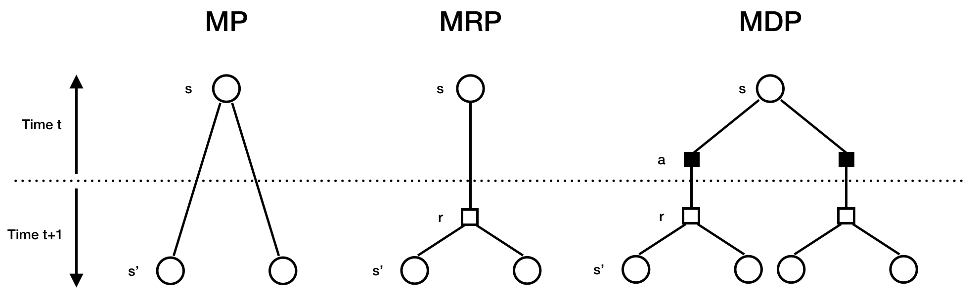
Visualization Summary of Different Processes

Appendix: Probability Review

Given the sample space $\Omega$ of a random quantity.

Event. It is a subset of $\Omega$

Random variable. It is a valued-function defined on $\Omega$, namely $X: \Omega\rightarrow?$

Expectation. $E\{X\}=\sum_{\omega\in\Omega}X(\omega)P(\omega)$

Expectation conditioned on event (Conditional expectation). $E\{X|E\}=\sum_{\omega\in E}X(\omega)P(\omega)$