Model-Free Prediction

Assumption:

1. unknown MDP. You know the states, but you don't know the transition probabilities and the reward function
2. All states must be visited enough times.

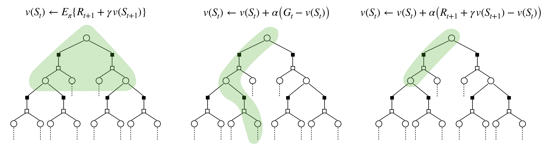
Goal. We want to perform policy evaluation. Recall that we have $v_\pi(s)=E_{\pi}\{G_t|S_t=s\}$ and $G_t=R_{t+1}+\gamma R_{t+2} + ... + \gamma^{T-1}R_T$.

Solution 1: Monte-Carlo - update after batch of episodes - (update only for first visit of state)

PSEUDOCODE

• Given a batch of episodes.
  • Count the number of times a state is visited for the first time in an episode , i.e. $N(s)$.
  • At the end of each episode compute the cumulative return for those visits, i.e. $S(s)$.
• After the whole batch of episodes, compute $v(s)=\frac{S(s)}{N(s)}$.

State-value function is estimated using empirical mean, namely $G_t=\frac{1}{N}\sum_{i=1}^N G_{t,i}$.
$G_t$ a Gaussian RV by central limit theorem and variance decreases as $1/N$.

Solution 2: Monte-Carlo - update after batch of episodes - (update for every visit of state)

PSEUDOCODE

• Given a batch of episodes.
  • Count the number of times a state is visited, i.e. $N(s)$.
  • At the end of each episode compute the cumulative return for those visits, i.e. $S(s)$.
• After the whole batch of episodes, compute $v(s)=\frac{S(s)}{N(s)}$.

Solution 3: Incremental Monte-Carlo - update after an episode

Note that given a sequence $x_1,x_2,\dots$, we can express the mean estimate in the following way: $$\begin{align}\mu_k &= \frac{1}{k}\sum_{i=1}^kx_i \\ &= \frac{1}{k}\big(x_k + \sum_{i=1}^{k-1}x_i\big) \\ &= \frac{1}{k}\big(x_k + (k-1)/(k-1)\sum_{i=1}^{k-1}x_i\big) \\ &= \frac{1}{k}\big(x_k + (k-1)\mu_{k-1}\big) \\ &= \mu_{k-1} + \frac{1}{k}\big(x_k -\mu_{k-1}\big) \end{align}$$

PSEUDOCODE

• Given a batch of episodes.
  • Count the number of times a state is visited (First/Every) , i.e. $N(s)$.
  • At the end of an episode compute $v(s)=v(s)+\frac{1}{N(s)}\big(G_t - v(s)\big)$

For non-stationary environment the update equation can be $v(s)=v(s)+\alpha\big(G_t - v(s)\big)$. Nevertheless, this is the solution used in practice.

Solution 4: Temporal-Difference Learning - complete online algorithm

Note that

\[\begin{align}v_\pi(s) &= E_\pi\{G_t|S_t=s\} \\ &=\sum_{a}\pi(a|s)\big(R_s^a + \gamma \sum_{s'}P_{ss'}^a E_\pi\{G_{t+1}|S_{t+1}=s'\}\big) \\ &=\sum_{a}\pi(a|s)\big(R_s^a + \gamma \sum_{s'}P_{ss'}^a v_\pi(s')\big)\end{align}\]

Therefore, if you observe $S_t,A_t,S_{t+1}$, then you can approximate $v(S_t)$ as $R_{t+1} + \gamma v(S_{t+1})$.

PSEUDOCODE

• After each single visit compute $v(S_t)=v(S_t)+\frac{1}{N(s)}\big([R_{t+1}+\gamma v(S_{t+1})] - v(S_t)\big)$.

$R_{t+1}+\gamma v(S_{t+1})$ is called TD target and $[R_{t+1}+\gamma v(S_{t+1})] - v(s)$ is called TD error.

Considerations (vs. Monte-Carlo)

1. TD can learn without final outcome (non-terminating or incomplete sequences)
2. TD can learn online
3. TD target has bias (because $v(S_{t+1})$ is a biased estimate of $v_\pi(S_{t+1})$) - MC is unbiased ($G_{t}$ is an unbiased of $v_\pi(S_t)$)
4. TD target has low variance (because it depends only on 1 action, 1 reward and 1 transition) - MC has high varaince (because it depends on all random subsequent steps).
5. Because of low variance, TD usually converges faster than MC.
6. TD converges to $v_\pi(s)$ (except in some cases when you use function approximation).
7. Because of bias, TD is sensitive to the initial starting point.

Analysis of Monte-Carlo and Temporal Difference

Question 1. Both MC and TD converge to the true value (when the number of episodes is large enough and you visit all states). What happens when the number of episodes is finite?
Answer. They can converge to different solutions.
Example: Consider a batch of episodes with 2 states, A and B (no discounting)

• B,1
• B,1
• B,1
• B,1
• B,1
• B,1
• B,0
• A,0,B,0

MC achieves $V(A)=0$ and $V(B)=6/8=3/4$, while TD achieves $V(A)=V(B)=3/4$. In fact, MC is the solution of the squared error objective $\sum_{e=episodes}\sum_{t=visit}(G_t^e-v(S_t^e))^2$, while TD first creates a Markov model and then solves the model. In fact, it implicitly estimates the transition probabilities and the reward function:

$$\hat{P}_{ss'}^a=\frac{1}{N(a,s)}\sum_{e=episodes}\sum_{t=visit}1[S_t^e,A_t^e,S_{t+1}^e=s,a,s']$$
$$\hat{R}_s^a=\frac{1}{N(a,s)}\sum_{e=episodes}\sum_{t=visit}1[S_t^e,A_t^e = s,a]R_{t+1}^e$$

This tells us that TD exploits the Markov property and it typically works better in Markov environments, while MC works better in non-Markov environments (like POMDPs).

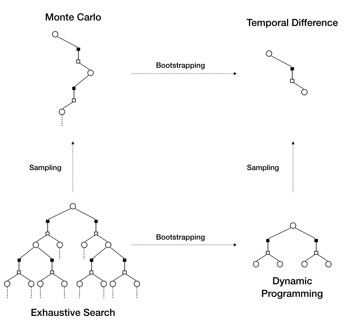
Question 2. Can we unify the methods?

Answer. Yes, let's consider Dynamic Programming, Monte-Carlo and Temporal Difference.

Define bootstrapping (making only 1 step ahead) and sampling (estimate the expectation)

We can unify Monte-Carlo and Temporal Difference, by considering intermediate look aheads. Define n-step return, namely $G_t^{(n)}=R_{t+1}+\gamma R_{t+2}+\dots+\gamma^{n-1}R_{t+n}+\gamma^nv(S_{t+n})$

PSEUDOCODE (n-step TD)

• After each single visit compute $v(S_t)=v(S_t)+\alpha\big(G_t^{(n)} - v(S_t)\big)$.

If $n=1$ we get normal TD, if $n\rightarrow\infty$ we get MC.
Which $n$ is the best? Combine all!
(Geometric average) Define the $\lambda$-return, namely $G_t^\lambda=(1-\lambda)\sum_{n=1}^\infty\lambda^{n-1}G_t^{(n)}$.

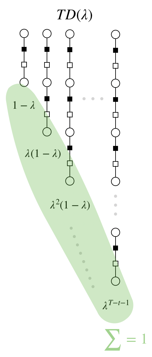
PSEUDOCODE (TD($\lambda$))

• After each episode compute $v(S_t)=v(S_t)+\alpha\big(G_t^{\lambda} - v(S_t)\big)$.

Question 3. How is it possible to run TD($\lambda$) online instead of waiting until the end of an episode like in incremental Monte-Carlo?
Answer. Define an eligibility trace, namely

$$E_0(s)=0$$
$$E_t(s)=\gamma\lambda E_{t-1}(s) + 1[S_t=s]$$

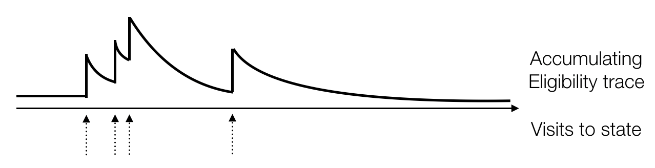
We can rewrite TD($\lambda$) in an online fashion

PSEUDOCODE (online TD($\lambda$))

• After each single visit compute $v(S_t)=v(S_t)+\alpha \delta_t E_t(s)$, where $\delta_t$ is the TD error, namely $\delta_t=R_{t+1}+\gamma v(S_{t+1})-v(S_t)$

Theorem. Assume you perform offline updates (namely, for online TD($\lambda$) you update the state-value function at the end of each episode). Then, the total update performed by online TD($\lambda$) is equivalent to the total update performed by TD($\lambda$). In fact,

$$\alpha\sum_{t=1}^T \delta_t E_t(s)=\alpha\sum_{t=1}^T\big(G_t^{\lambda}-v(S_t)\big)1[S_t=s]$$

Proof. We prove it just for the case in which state $s$ is visited once in the episode. Let's assume that the visit occurs at time $k$.
Recall the definition of eligibility trace, viz. $E_t(s)=\lambda\gamma E_{t-1}(s) + 1[s_t=s]$ and $E_0(s)=0$. Therefore, we have that for $t<k$, $E_t(s)=0$ and for $t\leq k$, $E_t(s)=(\lambda\gamma)^{t-k}$. Consequently, $\alpha\sum_{t=1}^T \delta_t E_t(s)=\alpha\sum_{t=k}^T \delta_t (\lambda\gamma)^{t-k}$. Furthermore, $\alpha\sum_{t=1}^T\big(G_t^{\lambda}-v(S_t)\big)1[S_t=s]=\alpha \big(G_k^{\lambda}-v(S_k)\big)$.
Therefore, we need to prove the following statement

$$\alpha\sum_{t=k}^T \delta_t (\lambda\gamma)^{t-k}=\alpha \big(G_k^{\lambda}-v(S_k)\big)$$

We prove this for $T=k+1$, namely

$$\sum_{t=k}^{k+1} \delta_t (\lambda\gamma)^{t-k}= \big(G_k^{\lambda}-v(S_k)\big)$$

Now

$$\begin{align}\sum_{t=k}^{k+1} \delta_t (\lambda\gamma)^{t-k} &=\delta_k + \delta_{k+1}\lambda\gamma \\ &= R_{k+1} + \gamma v(S_{k+1}) - v(S_k) + \lambda\gamma\big(R_{k+2} + \gamma v(S_{k+2}) - v(S_{k+1})\big) \\ &= R_{k+1} + \gamma v(S_{k+1}) - \lambda\gamma v(S_{k+1}) + \lambda\gamma\big(R_{k+2} + \gamma v(S_{k+2})\big) - v(S_k) \quad\text{ and now add }\quad -\lambda R_{k+1} + \lambda R_{k+1} \\ &= R_{k+1} + \gamma v(S_{k+1}) -\lambda R_{k+1} + \lambda R_{k+1} - \lambda\gamma v(S_{k+1}) + \lambda\gamma\big(R_{k+2} + \gamma v(S_{k+2})\big) - v(S_k) \\ &= R_{k+1} + \gamma v(S_{k+1}) -\lambda R_{k+1} - \lambda\gamma v(S_{k+1}) + \lambda R_{k+1} + \lambda\gamma\big(R_{k+2} + \gamma v(S_{k+2})\big) - v(S_k) \\ &= R_{k+1} + \gamma v(S_{k+1}) -\lambda \big(R_{k+1} + \gamma v(S_{k+1})\big) + \lambda R_{k+1} + \lambda\gamma\big(R_{k+2} + \gamma v(S_{k+2})\big) - v(S_k) \\ &= \big(1-\lambda\big)\big(R_{k+1} + \gamma v(S_{k+1})\big) + \lambda R_{k+1} + \lambda\gamma\big(R_{k+2} + \gamma v(S_{k+2})\big) - v(S_k) \\ &= \big(1-\lambda\big)\big(R_{k+1} + \gamma v(S_{k+1})\big) + \lambda\big(R_{k+1} + \gamma R_{k+2} + \gamma^2 v(S_{k+2})\big) - v(S_k) \\ &= \big(1-\lambda\big)G_k^{(1)} + \lambda G_k^{(2)} - v(S_k) \\ &= G_k^\lambda - v(S_k) \end{align}$$

QED

Final considerations.

1. if $\lambda=0$, then $G_t^{\lambda}=(1-\lambda)\sum_{n=1}^\infty\lambda^{n-1}G_t^{(n)}=G_t^{(1)}$. In other words, we recover TD.
2. if $\lambda=1$, then all terms except the last one in the summation of $G_t^{\lambda}$ cancel out. Therefore, we obtain $G_t^{\lambda}=G_t^{(T)}$, namely we recover MC.
3. Note that the paper of Sutton and von Seijen (ICML 2014), proposes a slightly different eligibility trace and prove the equivalence in the theorem even for online updates.