Exploration and Exploitation Dilemma

In this lecture, we study the dilemma of exploitation and exploration. Exploration aims at collecting information and exploitation aims at using the information to gain as much reward as possible.
The problem of exploration and exploitation can be analyzed in the multi-armed bandit setting, which is the most fundamental and simplest problem in reinforcement learning. The insights achieved by the theoretical analysis can be also helpful for more complex problems, like contextual bandits and full MDPs.

Multi-Armed Bandit

The multi-armed bandit problem is defined by the tuple $<A,R>$, where $A$ is a finite set of actions (or arms) and $R$ is the reward function. At each time step, an arm needs to be chosen and a reward is drawn from an unknown density $p(r|a)$. The agent must select the arm which maximizes the conditional expected reward.
We define the action-value function $q(a)=E\{R|A=a\}$ (note that the environment is equivalent to a 1-step MDP) and the optimal action is given by $a^*=\arg\max_a q(a)$.

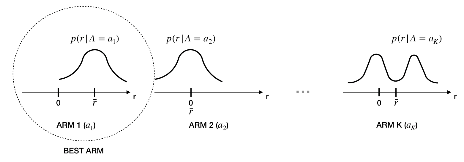
Unfortunately, the densities associated to each arm are unknown and the agent must be able to balance exploring new arms and exploiting the knowledge of already visited arms. In general, the agent incurs in a loss when taking decisions. We define the regret at time as $t$ $I_t=E\{q(a^*)-q(a_t)\}$ and the total regret as $L_t=E\{\sum_{\tau=1}^t q(a^*)-q(a_\tau)\}$.
Note that

$$\begin{align} L_t &= E\Big\{\sum_{\tau=1}^t q(a^*)-q(a_\tau)\Big\} \\ &= \sum_{a\in A}\big(q(a^*)-q(a)\big)E\{N_t(a)\} \quad\text{where}\quad N_t(a)=\text{# times action is picked} \\ &= \sum_{a\in A}\Delta_a E\{N_t(a)\} \quad\text{where}\quad \Delta_a=\big(q(a^*)-q(a)\big)\text{ is called gap} \end{align}$$

Minimizing the total regret consists of picking more frequently actions with low gap. The total regret is an indicator which tells which algorithm is able to explore/exploit optimally.

Algorithm Analysis: Greedy Algorithms

A greedy algorithm has two steps:

1. Action-value estimation, through Monte-Carlo estimation $Q_t(a)=\frac{1}{N_t(a)}\sum_{\tau=1}^t1[a_\tau=a]r_\tau$.
2. Choose arm greedily $a_t=\arg\max_a Q_t(a)$

Note that greedy algorithms incur in linear total regret. Once a wrong action is taken, the algorithm can continue to pick that action, thus adding the same gap at each timestep. To understand this phenomenon consider the following example

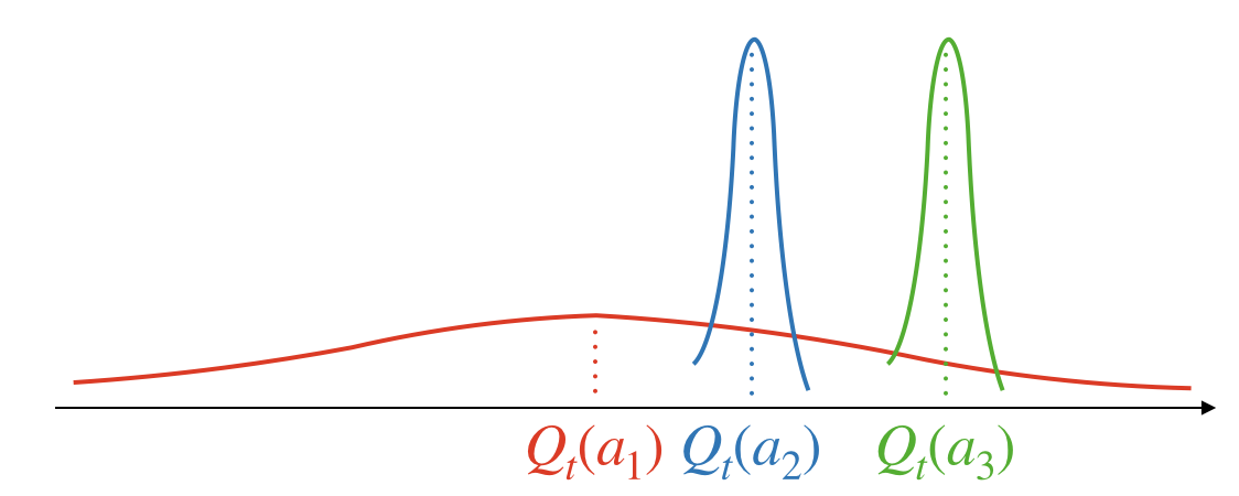
Suppose that there are three arms $a_1,a_2,a_3$ and that

1. $a_1$ is the optimal arm visited only few times
2. $a_2$ and $a_3$ are visited many times

Now, the greedy algorithm performs a Monte-Carlo estimate of the average reward for each arm. This estimate has lower variance for frequently visited arms than rarely visited ones (see the curves for each arm in the picture). Note that the algorithm chooses the arm greedily and it always selects arm $a_3$. This choice is suboptimal.

Algorithm Analysis: $\epsilon$-Greedy Algorithms

A common strategy is to introduce random exploration in the arm selection stage. In fact, we can pick a random arm with probability $\epsilon$ and pick arm $a_t=\arg\max_a Q_t(a)$ with probability $1-\epsilon$.
This strategy avoids to get stuck to selecting wrong arms. Nevertheless, it is suboptimal because noise is introduced at each time step. To understand this, consider previous example. Action $a_2$ can be selected even though we are almost sure that it is not optimal and therefore we are wasting decisions.
Note that

$$E\{N_t(a)\}=\frac{\epsilon t}{|A|-1}\geq\frac{\epsilon t}{|A|}$$

Therefore (by recalling the relation between total regret and the total number of visits for arm $a$)

$$L_t\geq \frac{\epsilon t}{|A|}\sum_{a\in A}\Delta_a$$

Therefore, greedy algorithms incur in linear total regret.

Question. Can we do better?
Yes, one strategy is to perform optimistic initialization (all actions are initially good) and then we can act greedily. This is a trick that works particularly well in practice, but it has no theoretical guarantee on the performance.
Yes, we can also decay $\epsilon$, but in general it is difficult to devise a theoretically grounded strategy for decaying it.

Question. Can we do better by guaranteeing a sublinear total regret?

Algorithm Analysis: Optimal Algorithm

In 1985 Lai and Robbins showed that the total regret of any algorithm for the multi-armed bandit can be lower bounded, namely:

$$E\{N_t(a)\}\geq\frac{\log t}{KL\big\{p(r|A=a)||p(r|A=a^*)\big\}} \quad\text{for}\quad t\rightarrow\infty$$

and therefore (by recalling the relation between total regret and the total number of visits for arm $a$)

$$L_t\geq \log t\sum_{a\neq a^*}\frac{\Delta_a}{KL\big\{p(r|A=a)||p(r|A=a^*)\big\}} \quad\text{for}\quad t\rightarrow\infty$$

The optimal algorithm achieves an asymptotical logarithmic total regret.

Question. How can we achieve that?
The answer can be obtained by considering the example described above. Note that, the most uncertain action $a_1$ has the biggest potential to be the optimal one (the tail on the right is the highest one), whereas we can confidently say that action $a_2$ is likely to be worse than action $a_3$ as the estimates differ and have low variance. Therefore, we can balance exploration and exploitation by taking into account the estimates together with their uncertainty.

Algorithm Analysis: Upper Confidence Bound (UCB)

Instead of considering only the estimate of the action-value function, we can consider an upper bound on the estimate and ensure that the true value is smaller than the bound with very high probability.

At this purpose, we can recall the Hoeffding's inequality.

Hoeffding's inequality. Given a random variable $X$ defined on the $[0,1]$ sample space. If we get an i.i.d set of samples $x_1,...,x_t$ and define the sample mean $\bar{x}_t=\frac{1}{t}\sum_{\tau=1}^tx_\tau$, then

$$P\big(E\{X\}>\bar{x}_t+u\big)\leq e^{-2tu^2}$$

Now, we can use it for our estimates. In fact, assume that the reward is defined on $[0,1]$, we have that $Q_t(a)=\frac{1}{N_t(a)}\sum_{\tau=1}^t1[a_\tau=a]r_\tau$. Therefore,

$$P\big(q(a)>Q_t(a)+U_t(a)\big)\leq e^{-2N_t(a)U_t(a)^2}$$

We define probability $p=e^{-2N_t(a)U_t(a)^2}$, then we get that $U_t(a)=\sqrt{\frac{-\log p}{2N_t(a)}}$.
And by decreasing $p$ over time (in order to ensure that the true value is finally included with certainty), e.g. $p=t^{-4}$, we obtain that

$$U_t(a)=\sqrt{\frac{2\log t}{N_t(a)}}$$

The UCB algorithm selects actions according to the followig rule:

$$a_t=\arg\max_a Q_t(a)+\sqrt{\frac{2\log t}{N_t(a)}}$$

The paper of Auer et al. 2002 proves that the UCB algorithm satisfies the following bound, namely:

$$E\{N_t(a)\}\leq\frac{8\log t}{\Delta_a^2}+c_1 \quad\text{for any }t$$

where $c$ is a small constant. Therefore (by recalling the relation between total regret and the total number of visits for arm $a$)

$$L_t\leq 8\log t\sum_{a\neq a^*}\frac{1}{\Delta_a}+c_2 \quad\text{for any }t$$

where $c_2$ is a small constant. UCB achieves logarithmic total regret.
The algorithm is not optimal though as the proved bound is worse than the one proved by Lai and Robbins. In fact, you can prove that $KL\{p(r|A=a)||p(r|A=a^*)\}\geq 2\Delta_a^2$, in other words that $\frac{1}{KL\{p(r|A=a)||p(r|A=a^*)\}}\leq \frac{0.5}{\Delta_a^2}$. Therefore, $\frac{1}{KL\{p(r|A=a)||p(r|A=a^*)\}}\leq \frac{0.5}{\Delta_a^2}<\frac{8}{\Delta_a^2}$. The paper of Auer et al. 2002 provides more sophisticated strategies than the UCB algorithm, improving the constant $8$ in the bound by getting closer to $0.5$ (see the paper for further details).

Algorithm Analysis: Bayesian Upper Confidence Bound

(FOR SCALAR REWARDS)

Note that our aim is to compute an estimate of the true value $q(a)$ given a set of observations of rewards. Let's define $\bar{r}_a=q(a)$ and $\hat{r}_a$ as the sample mean estimate of the true value $\bar{r}_a$. $\hat{r}_a$ is a random quantity and we can assume that it has Gaussian density (by considering that $\bar{r}_a$ is a sample mean estimate and by using the central limit theorem for sufficiently large number of such samples).
Therefore, we define $p(\hat{r}_a|\mu_a,\sigma_a^2)=\mathcal{N}(\hat{r}_a;\mu_a,\sigma_a^2)$ and a prior $p(\mu_a,\sigma_a^2)$ (which is typical uniform).
Given the set of all rewards observed up to time $t$ for action $a$,viz. $D_t^a$, the algorithm performs the following steps:

1. Compute the posterior for time $t$
   \[\begin{align}p(\mu_a,\sigma_a^2|D_t^a) &= \frac{p(D_t^a|\mu_a,\sigma_a^2)p(\mu_a,\sigma_a^2)}{Z} \\ &\propto p(D_t^a|\mu_a,\sigma_a^2)p(\mu_a,\sigma_a^2) \\ &= \prod_{r\in D_t^a}p(\hat{r}_a=r|\mu_a,\sigma_a^2) \\ &= \prod_{r\in D_t^a}\mathcal{N}(\hat{r}_a=r;\mu_a,\sigma_a^2)p(\mu_a,\sigma_a^2) \end{align}\]
   
2. Get $\mu_a$ and $\sigma_a$
3. Select arm according to $$a_{t+1}=\arg\max_a \mu_a+c\sigma_a$$ where $c$ is an arbitrary positive integer.

This algorithm is optimal for sufficiently large number of visits for action $a$ and for specific choices of $c$. Nevertheless, there are solutions which do not require setting any hyperparameter.

Algorithm Analysis: Thompson Sampling

Assume that we have:

• a set of observations $D=\{(a_1,r_1),\dots,(a_t,r_t)\}$
• a parametric reward probability $p(r|a,\theta)$
• a prior over parameters, $p(\theta)$

Note that greedy algorithms attempt to maximize

$$\begin{align} q(a) &= E\{R|A=a,D\} \\ &= \int r p(r|A=a,D) dr \\ &= \int r \int p(r|A=a,D,\Theta=\theta)p(\theta|A=a,D) d\theta dr \\ &= \int \int r p(r|A=a,D,\Theta=\theta) dr p(\theta|A=a,D) d\theta \\ &= \int E\{R|A=a,D,\Theta=\theta\}p(\theta|A=a,D)d\theta \end{align}$$

Thompson sampling approaches the problem differently, in the sense that it attempts to estimate $p(a\text{ is optimal}|D)$ and maximize it. In fact,

$$\begin{align} p(a\text{ is optimal}|D) &= \int p(a\text{ is optimal},\Theta=\theta|D) d\theta \\ &= \int p(a\text{ is optimal}|\Theta=\theta,D) p(\theta|D) d\theta \\ &= \int 1\big[E\{R|A=a,\Theta=\theta,D\}=\max_{a'}E\{R|A=a',\Theta=\theta,D\}\big]p(\theta|D) d\theta \end{align}$$

Basically, this integral performs a partition of the parameter space $\Theta$ (where each region has its own optimal actions) and uses the posterior $p(\theta|D)$ to compute $p(a\text{ is optimal}|D)$ for all $a$. See the following picture for an example of 2 dimensional parameter space

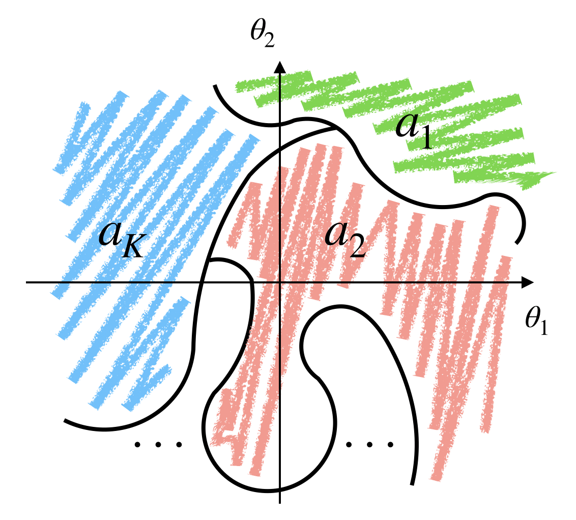
Computing the integral is usually intractable. Therefore, one can

1. Compute the posterior $p(\theta|D)$.
2. Sample $\theta$ (or get a bunch of samples) from the posterior $p(\theta|D)$.
3. Compute $E\{R|A=a,\Theta=\theta,D\}$ for all $a$.
4. Choose with probability 1 the action corresponding to the highest $E\{R|A=a,\Theta=\theta,D\}$.

Note that these steps are different from greedy algorithms. In fact, we choose action $a$ proportionally to its probability of being optimal (in other words we perform probability matching).
To better understand the difference with respect to greedy algorithms, let's consider the case of binary rewards (Bernouilli bandits). In this case, we have that $p(\theta|D)=\prod_{a\in A}p(\theta_a|D)$.
In greedy algorithms, we have that

$$\begin{align} q(a) &= E\{R|A=a,D\} \\ &= \sum_{r\in\{0,1\}}r \int Be(r|\theta_a)p(\theta_a|D) d\theta_a \\ &= \int \theta_a p(\theta_a|D) d\theta_a \quad\text{as}\quad \theta_a=p(r=1|A=a,D)\\ \end{align}$$
and we choose the arm with highest mean value of parameter posterior (we compute an expectation over the whole parameter space).
In Thompson sampling, we maximize
$$p(a\text{ is optimal}|D)=\int 1\big[\theta_a=\max_{a'}\theta_a'\big]p(\theta_a|D) d\theta_a$$
In this case, we integrate only on the region of the parameter space for which the arm is optimal. Note that Thompson sampling achieves logarithmic total regret in Bernouilli bandits.

Algorithm Analysis: Algorithms based on Information State

Assume that we have:

• a parametric reward probability $p(r|a,\theta)$
• a conjugate prior over parameters, $p(\theta)$

An information state is defined to capture all information available so far. In the case of Bernouilli bandits, the reward probability is a Bernouilli distribution $Be(\theta_a)$ and the parameter prior is the Beta distribution $B(\alpha_a,\beta_a)$. The information state is defined as the vector containing the hyperparameters of the Beta prior, namely $\tilde(s)=[\alpha_1,\beta_1,\dots,\alpha_K,\beta_K]$.

By using the definition of information state, we can define a MDP, namely $<\tilde{S},A,\tilde{P},R,\gamma>$. Note that in the case of conjugate priors, the hyperparameters can be computed in closed form (for example in Bernouilli bandits $\alpha_a\leftarrow\alpha_a+1$ if $r=1$ and $\beta_a\leftarrow\beta_a+1$ if $r=0$). This is important because we know the transition probability $\tilde{P}$ and we can use dynamic programming to find the optimal strategy. For this reasons, algorithms based on information state are optimal to balance exploration and exploitation.

If dynamic programming cannot be used, we can use other RL algorithms (that we have already introduced in previous lectures).

Contextual Bandit

A contextual bandit is a tuple $<A,S,R>$, where

• we have an unknown density over states $p(s)$
• we have a density for rewards $p(R=r|S=s,A=a)$

Note that a contextual bandit introduces states compared to multi-armed bandits. Furthermore, it differs from the full RL setting, as the states are not influenced by any action or previous state (therefore we don't have a transition probability between states).

Contextual bandits have been used for personalized web advertising. Each state is used to describe the specific preferences of each user, actions are used to select which advertising to display to the user and rewards consists of advertising clicks made by each user.

Example from Paper
Consider the following setting:

• a linear reward model $r_s^a=\phi(s,a)^T\mu, \phi(s,a)^T\Sigma\phi(s,a)\theta$
• Gaussian prior over the parameters $\theta\sim\mathcal{N}(\mu,\Sigma)$ with diagonal $\Sigma$
• a dataset of observations $D=\{(s_1,a_1,r_1),\dots,(s_T,a_T,r_T)\}$

Then, we know that $r$ is a linear transformation of random vector $\theta$, thus $r_s^a\sim\mathcal{N}\big(\phi(s,a)^T\mu, \phi(s,a)^T\Sigma\phi(s,a)\big)$.
The proposed algorithm maximizes the following objective with respect to $\mu,\Sigma$

$$\begin{align} \log p(D|\mu,\Sigma) &= \log\prod_{i=1} p(s_i,a_i,r_i|\mu,\Sigma) \\ &= \sum_{i=1}\log p(r_i|s_i,a_i;\mu,\Sigma)p(s_i,a_i) \quad\text{consider uniform prior} \\ &= \sum_{i=1}\log p(r_i|s_i,a_i;\mu,\Sigma) \\ &= \sum_{i=1}\log \mathcal{N}\big(\phi(s_i,a_i)^T\mu, \phi(s_i,a_i)^T\Sigma\phi(s_i,a_i)\big) \end{align}$$

Afterwards, it selects actions for given state $s'$ by using the following upper confidence bound

$$\begin{align} a^* &= \arg\max_a \phi(s',a)^T\mu^* + c\sqrt{\phi(s',a)^T\Sigma^*\phi(s',a)} \end{align}$$

Full MDPs

The same principles used in multi-armed bandits can be applied to the full MDP problem. Please, see the slides of David Silver for further details on this.

Final Remarks

It is important to mention that there are other factors that have to be considered when dealing with exploration and exploitation. For example, in extremely large state spaces it is not possible to explore all possible states. Therefore, we need to decide which subset of states to explore. Another example consists of safety-concerned applications, where state exploration must provide some safety guarantees.