Value Function Approximation

Note that in many interesting real-world applications the number of states is very large. For example, in backgammon the number of states is in the order of $10^{20}$, in Computer Go is in the order of $10^{170}$ and in helicopter we have a continuous state space and therefore the number is uncountably infinite.
In such scenarios, we have two problems:

1. Memory. In fact, it could be not possible to store the values for each state or for each actio-state pair.
2. Inefficient Learning. It is very inefficient to learn the value of each state independently (they are not independent).

Solution. Use a function approximator. For each state or action-state pair, you can compute the corresponding value without storing it. Furthermore, the parameters of the function approximator are in general much less than the number of states, this allows for capturing the dependence between states and generalize to unseen states.

$$\hat{v}(s;w)\approx v_\pi(s)$$
$$\hat{q}(a,s;w)\approx q_\pi(a,s)$$

There are three kinds of function approximator.

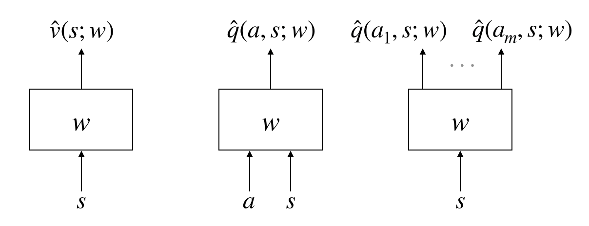
Question. How can we learn such function approximators?
Answer. Through supervised learning.
There are mainly two categories, namely incremental methods and batch methods. Incremental methods use samples, perform updates and throw away them, whereas batch methods store samples and reuse them.

Incremental methods: Prediction

Imagine that for a policy $\pi$, we can access a sequence of training pairs, namely:

$$\big(S_1,v_\pi(S_1)\big),\big(S_2,v_\pi(S_2)\big),\dots,\big(S_t,v_\pi(S_t)\big),\dots$$

Now, for a specific state $s$, we can compute the following ojective, called Mean Squared Value Error (MSVE)

$$\begin{align}J(w)&=\frac{1}{2}E\big\{\big(v_\pi(s)-\hat{v}(s;w)\big)^2\big\} \\ &=\frac{1}{2}\sum_s p(s)E\big\{\big(v_\pi(S_t)-\hat{v}(S_t;w)\big)^2|S_t=s\big\}\end{align}$$

Then, we can learn by SGD

$$\begin{align}\Delta w &= \alpha E\big\{\big(v_\pi(s)-\hat{v}(s;w)\big)\nabla_w \hat{v}(s;w)\big\} \\ &\approx \alpha\big(v_\pi(s)-\hat{v}(s;w)\big)\nabla_w \hat{v}(s;w)\end{align}$$

where the last step is computed using a finite sequence of training pairs (an episode of policy $\pi$).
Problem. This sequence is not available in practice as $v_\pi(\cdot)$ is not known.

Solution 1: Monte Carlo with Function Approximation

Now the sequence is

$$\big(S_1,G_1\big),\big(S_2,G_2\big),\dots,\big(S_t,G_t\big),\dots,\big(S_t,G_T\big)$$

and the update is given by

$$\begin{align}\Delta w &\approx \alpha\big(G_t-\hat{v}(s;w)\big)\nabla_w \hat{v}(s;w)\end{align}$$

Theorem. Monte Carlo with Function Approximation finds an unbiased estimate of the true state-value function.
Proof. The objective for Monte Carlo with Function Approximation is given by the Mean Squared Return Error (MSRE), namely:

$$\begin{align}J(w)&=E\big\{\big(G_t-\hat{v}(s;w)\big)^2\big\} \\ &=\sum_s p(s)E\big\{\big(G_t-\hat{v}(S_t;w)\big)^2|S_t=s\big\} \\ &=\sum_s p(s)E\big\{\big(G_t-v_\pi(S_t)-\text{error}(S_t;w)\big)^2|S_t=s\big\} \\ &=\sum_s p(s)E\big\{\big(G_t-v_\pi(S_t)\big)^2-2\big(G_t-v_\pi(S_t)\big)\text{error}(S_t;w)+\text{error}(S_t;w)^2|S_t=s\big\} \\ &=\sum_s p(s)\bigg[E\big\{\big(G_t-v_\pi(S_t)\big)^2|S_t=s\big\}-2E\big\{\big(G_t-v_\pi(S_t)\big)\text{error}(S_t;w)|S_t=s\big\}+E\big\{\text{error}(S_t;w)^2|S_t=s\big\}\bigg] \\ &=\sum_s p(s)\bigg[E\big\{\big(G_t-v_\pi(S_t)\big)^2|S_t=s\big\}-2E\big\{\big(G_t-v_\pi(S_t)\big)|S_t=s\big\}E\big\{\text{error}(S_t;w)|S_t=s\big\}+E\big\{\text{error}(S_t;w)^2|S_t=s\big\}\bigg] \\ &=\sum_s p(s)\bigg[E\big\{\big(G_t-v_\pi(S_t)\big)^2|S_t=s\big\}+E\big\{\text{error}(S_t;w)^2|S_t=s\big\}\bigg] \\ &=\sum_s p(s)\bigg[E\big\{\big(G_t-v_\pi(S_t)\big)^2|S_t=s\big\}+E\big\{\big(v_\pi(S_t)-\hat{v}(S_t;w)\big)^2|S_t=s\big\}\bigg] \\ &=\sum_s p(s)\bigg[E\big\{\big(G_t-v_\pi(S_t)\big)^2|S_t=s\big\}\bigg]+\sum_s p(s)\bigg[E\big\{\big(v_\pi(S_t)-\hat{v}(S_t;w)\big)^2|S_t=s\big\}\bigg] \\ &=\sum_s p(s)\bigg[E\big\{\big(G_t-v_\pi(S_t)\big)^2|S_t=s\big\}\bigg]+MSVE(w) \\ \end{align}$$

Note that the first term doesn't depend on $w$. Therefore, minimizing MSRE is equivalent to minimize MSVE. The solution is an unbiased estimate. QED

Solution 2: Temporal Difference Learning with Function Approximation

Now the sequence is

$$\big(S_1,R_2+\gamma\hat{v}(S_2;w)\big),\big(S_2,R_3+\gamma\hat{v}(S_3;w)\big),\dots,\big(S_t,R_{t+1}+\gamma\hat{v}(S_{t+1};w)\big),\dots$$

and the update is given by

$$\begin{align}\Delta w &\approx \alpha\big(R_{t+1}+\gamma\hat{v}(S_{t+1};w)-\hat{v}(s;w)\big)\nabla_w \hat{v}(s;w)\end{align}$$

Problem. There is no equivalent objective function from which we can derive this update formula. In this case, the updates are performed online (not exactly supervised learning).
This is a heuristic method with no guarantee about convergence to optimal solution. Furthermore, there are counterexamples showing that this method can diverge. It has been used in many practical cases.

Solution 3: TD($\lambda$) Learning with Function Approximation

Now the sequence is

$$\big(S_1,G_1^\lambda\big),\big(S_2,G_2^\lambda\big),\dots,\big(S_t,G_t^\lambda\big),\dots,\big(S_t,G_T^\lambda\big)$$

and the update is given by

$$\begin{align}\Delta w &\approx \alpha\big(G_t^\lambda-\hat{v}(s;w)\big)\nabla_w \hat{v}(s;w)\end{align}$$

Problem. There is no equivalent objective function from which we can derive this update formula. Nevertheless, it tradeoffs MC and TD

Solution 4: Online TD($\lambda$) Learning with Function Approximation

Equivalently, we can introduce eligibility traces to make convert TD($\lambda$) to be online.
Nevertheless, the definition is different as the eligibility trace is defined on the parameters of the function approximator rather that the states, namely:

$$E_0=0$$
$$E_t=\gamma\lambda E_{t-1}+\nabla_w \hat{v}(S_t;w)$$

and the update rule is

$$\begin{align}\Delta w &\approx \alpha\big(R_{t+1}+\gamma\hat{v}(S_{t+1};w)-\hat{v}(s;w)\big)E_t\end{align}$$

Problem. As for TD($\lambda$), there is no equivalent objective function from which we can derive this update formula. Nevertheless, it tradeoffs MC and TD.

More Advanced Online Solutions

Solution 5: Residual Gradient with Function Approximation

Assumption. Assume that the function approximation can learn the true state-value function.
In order to have an online solution, we can use the Bellman Error as an objective. In fact, let's consider the Mean Squared Bellman Error (MSBE), namely:

$$\begin{align}J(w)&=\frac{1}{2}\sum_s p(s)\bigg[E\big\{\big(R_{t+1}^{S_t}+\gamma\hat{v}(S_{t+1};w)\big)|S_t=s\big\}-\hat{v}(s;w)\bigg]^2\end{align}$$

Now by computing the negative gradient, we obtain

$$\begin{align}\Delta w &= \alpha \sum_s p(s)\bigg[E\big\{\big(R_{t+1}^{S_t}+\gamma\hat{v}(S_{t+1};w)\big)|S_t=s\big\}-\hat{v}(s;w)\bigg]\bigg[\nabla_w \hat{v}(s;w)-\gamma E\big\{\nabla_w\hat{v}(S_{t+1};w)\big)|S_t=s\big\}\bigg] \\ &\approx \alpha \big(R_{t+1}^{s}+\gamma\hat{v}(s';w)-\hat{v}(s;w)\big)\big(\nabla_w \hat{v}(s;w)-\gamma \nabla_w\hat{v}(s^{''};w)\big)\end{align}$$

Note that in order to compute an unbiased estimate of the gradient, we need to sample two successor states, namely $s'$ and $s''$.
Note also that the update rule corresponds to TD update rule + a gradient correction term.
Problem. This solution is not optimal if the main assumption does not hold.

Solution 6: TD with Gradient Descent Methods and Linear Function Approximation

Assumption. There is no previous assumption. Therefore, this is the most general case.
Firstly, we have to define a projection operator. See the following picture to understand:

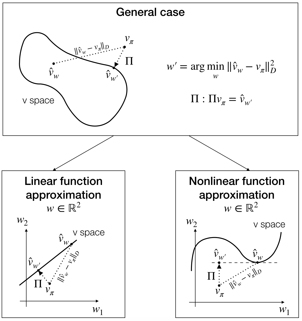
Formally,

$$\Pi: \Pi v_\pi = \hat{v}_{w'}$$

where

$$w'=\arg\min_w\|\hat{v}_{w}-v_\pi\|_D^2$$

and

$$D=\left[\begin{array}{llll}p(s_1)&&&\\ &p(s_2)&&\\ &&\ddots&\\ &&&p(s_{|S|})\end{array}\right]$$

In this case, we are considering the space of linear function approximators, $\hat{v}_{w}=\phi w$ where $\phi\in\mathbb{R}^{|S|\times d}$. Now, let's compute $w'$

$$\|\hat{v}_{w}-v_\pi\|_D^2 = \|\phi w-v_\pi\|_D^2=\big(\phi w-v_\pi\big)^TD\big(\phi w-v_\pi\big)=w^T\phi^TD\phi w-2w^T\phi^TDv_\pi+v_\pi^TDv_\pi$$

We can easily compute the minimum with respect to $w'$. In fact, $w'=\big(\phi^TD\phi\big)^{-1}\phi^TDv_\pi$. Now, let's use the definition of projection operator

$$\Pi v_\pi = \hat{v}_{w'}$$
$$\Pi v_\pi = \phi w'$$
$$\Pi v_\pi = \phi\big(\phi^TD\phi\big)^{-1}\phi^TDv_\pi$$

Therefore,

$$\Pi = \phi\big(\phi^TD\phi\big)^{-1}\phi^TD$$

Now, we are ready to define the Mean Squared Projected Bellman Error (MSPBE). Since, we don't have access to $v_\pi$, we can still have an indication where it is by exploiting the Bellman operator $T\hat{v}(s;w)=R_{t+1}^s+\gamma E\{\hat{v}(S_{t+1};w)|S_t=s\}$ (which points in the direction where $v_\pi$ is, as we know that the Bellman operator is contraction mapping and the convergence is linear). See the left picture

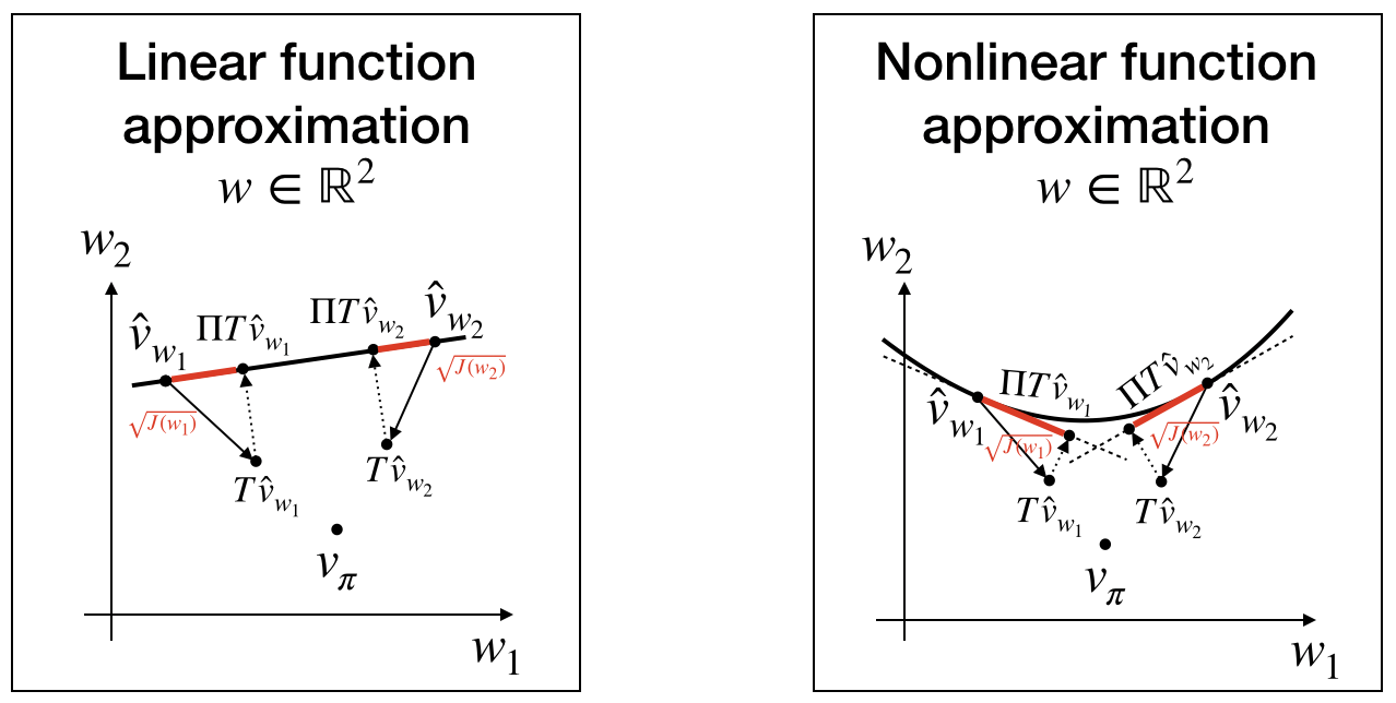
$$\begin{align}J(w)&=\frac{1}{2}\sum_s p(s)\bigg[\hat{v}(s;w)-\Pi_{s:}T\hat{v}(:;w)\bigg]^2\\ &=\frac{1}{2}\sum_s p(s)\bigg[\Pi_{s:}\hat{v}(:;w)-\Pi_{s:}T\hat{v}(:;w)\bigg]^2 \quad\text{as the point is projected to itself}\quad \hat{v}(s;w)=\Pi_{s:}\hat{v}(:;w) \\ &=\frac{1}{2}\sum_s p(s)\bigg[\Pi_{s:}\big(\hat{v}(:;w)-T\hat{v}(:;w)\big)\bigg]^2 \\ &=\frac{1}{2}\big(\hat{v}(:;w)-T\hat{v}(:;w)\big)^T\Pi^T D \Pi \big(\hat{v}(:;w)-T\hat{v}(:;w)\big) \\ &=\frac{1}{2}\big(\hat{v}(:;w)-T\hat{v}(:;w)\big)^T\big(\phi\big(\phi^TD\phi\big)^{-1}\phi^TD\big)^T D \big(\phi\big(\phi^TD\phi\big)^{-1}\phi^TD\big) \big(\hat{v}(:;w)-T\hat{v}(:;w)\big) \quad\text{by using}\quad \Pi = \phi\big(\phi^TD\phi\big)^{-1}\phi^TD \\ &=\frac{1}{2}\big(\hat{v}(:;w)-T\hat{v}(:;w)\big)^T\big(D^T\phi\big(\phi^TD\phi\big)^{-1}\phi^T\big) D \big(\phi\big(\phi^TD\phi\big)^{-1}\phi^TD\big) \big(\hat{v}(:;w)-T\hat{v}(:;w)\big) \\ &=\frac{1}{2}\big(\hat{v}(:;w)-T\hat{v}(:;w)\big)^TD^T\phi\big(\phi^TD\phi\big)^{-1}\big(\phi^T D \phi\big)\big(\phi^TD\phi\big)^{-1}\phi^TD \big(\hat{v}(:;w)-T\hat{v}(:;w)\big) \\ &=\frac{1}{2}\big(\hat{v}(:;w)-T\hat{v}(:;w)\big)^TD^T\phi\big(\phi^TD\phi\big)^{-1}\phi^TD \big(\hat{v}(:;w)-T\hat{v}(:;w)\big) \\ &=\frac{1}{2}\bigg[\phi^TD\big(\hat{v}(:;w)-T\hat{v}(:;w)\big)\bigg]^T\big(\phi^TD\phi\big)^{-1}\bigg[\phi^TD \big(\hat{v}(:;w)-T\hat{v}(:;w)\big)\bigg] \\ &=\frac{1}{2}\big(\phi^TD\delta_w\big)^T\big(\phi^TD\phi\big)^{-1}\big(\phi^TD \delta_w\big) \quad\text{where}\quad \delta_w=\big(\hat{v}(:;w)-T\hat{v}(:;w)\big) \\ &=\frac{1}{2}\big(\sum_s p(s)\delta_w(s)\phi_{s:}^T\big)^T\big(\phi^TD\phi\big)^{-1}\big(\sum_s p(s)\delta_w(s)\phi_{s:}^T\big) \\ &=\frac{1}{2}\bigg(\sum_s p(s)\big(\hat{v}(s;w)-T\hat{v}(s;w)\big)\phi_{s:}^T\bigg)^T\big(\sum_s p(s)\phi_{s:}^T\phi_{s:}\big)^{-1}\bigg(\sum_s p(s)\big(\hat{v}(s;w)-T\hat{v}(s;w)\big)\phi_{s:}^T\bigg) \\ &=\frac{1}{2}E_s\bigg\{\big(\hat{v}(s;w)-T\hat{v}(s;w)\big)\phi_{s:}^T\bigg\}^TE_s\bigg\{\phi_{s:}^T\phi_{s:}\bigg\}^{-1}E_s\bigg\{\big(\hat{v}(s;w)-T\hat{v}(s;w)\big)\phi_{s:}^T\bigg\} \end{align}$$

Now, we can take the gradient with respect to $w$, but first let's recall that

$$\nabla_w J(w)=\frac{1}{2}\nabla_w f(w)^T A f(w)=\text{Jac}\big(f(w)\big)^TA^Tf(w)$$

where $A=E_s\bigg\{\phi_{s:}^T\phi_{s:}\bigg\}^{-1}$ and $f(w)=\sum_s p(s)\big(\hat{v}(s;w)-T\hat{v}(s;w)\big)\phi_{s:}^T$

$$\begin{align} \text{Jac}\big(f(w)\big)=\sum_s p(s)\text{Jac}\big(\big(\hat{v}(s;w)-T\hat{v}(s;w)\big)\phi_{s:}^T\big) &= \sum_s p(s)\left[\begin{array}{lll} \frac{\partial\big(\hat{v}(s;w)-T\hat{v}(s;w)\big)\phi_{s1}}{\partial w_1} & \dots & \frac{\partial \big(\hat{v}(s;w)-T\hat{v}(s;w)\big)\phi_{s1}}{\partial w_d} \\ \vdots & & \vdots \\ \frac{\partial\big(\hat{v}(s;w)-T\hat{v}(s;w)\big)\phi_{sd}}{\partial w_1} & \dots & \frac{\partial\big(\hat{v}(s;w)-T\hat{v}(s;w)\big)\phi_{sd}}{\partial w_d} \end{array}\right] \\ &=\sum_s p(s)\phi_{s:}^T \bigg(\nabla_w\big(\hat{v}(s;w)-T\hat{v}(s;w)\big)\bigg)^T \\ &=\sum_s p(s)\phi_{s:}^T \bigg(\nabla_w\big(\hat{v}(s;w)-R_{t+1}^s-\gamma E\{\hat{v}(S_{t+1};w)|S_t=s\}\big)\bigg)^T \\ &=\sum_s p(s)\phi_{s:}^T \bigg(\nabla_w\hat{v}(s;w)-\gamma E\{\nabla_w\hat{v}(S_{t+1};w)|S_t=s\}\bigg)^T \\ &=\sum_s p(s)\phi_{s:}^T \bigg(\nabla_w\phi_{s:}w-\gamma E\{\nabla_w\phi_{S_{t+1}:}w|S_t=s\}\bigg)^T \\ &=\sum_s p(s)\phi_{s:}^T \bigg(\phi_{s:}^T-\gamma E\{\phi_{S_{t+1}:}^T|S_t=s\}\bigg)^T \\ &=\sum_s p(s)\phi_{s:}^T \bigg(\phi_{s:}-\gamma E\{\phi_{S_{t+1}:}|S_t=s\}\bigg) \\ &=\sum_s p(s)\phi_{s:}^T \bigg(\phi_{s:}-\gamma E_{s'|s}\{\phi_{s':}\}\bigg) \quad\text{to simplify notation}\\ &=E_s\bigg\{\phi_{s:}^T \big(\phi_{s:}-\gamma E_{s'|s}\{\phi_{s':}\}\big)\bigg\} \end{align}$$

Therefore,

$$\begin{align} \nabla_w J(w) &= E_s\bigg\{\phi_{s:}^T \big(\phi_{s:}-\gamma E_{s'|s}\{\phi_{s':}\}\big)\bigg\}^TE_s\bigg\{\phi_{s:}^T\phi_{s:}\bigg\}^{-1}E_s\bigg\{\big(\hat{v}(s;w)-T\hat{v}(s;w)\big)\phi_{s:}^T\bigg\} \\ &= E_s\bigg\{\phi_{s:}^T \big(\phi_{s:}-\gamma E_{s'|s}\{\phi_{s':}\}\big)\bigg\}^TE_s\bigg\{\phi_{s:}^T\phi_{s:}\bigg\}^{-1}E_s\bigg\{\delta_w(s)\phi_{s:}^T\bigg\} \\ &= E_s\bigg\{\big(\phi_{s:}-\gamma E_{s'|s}\{\phi_{s':}\}\big)^T \phi_{s:}\bigg\}E_s\bigg\{\phi_{s:}^T\phi_{s:}\bigg\}^{-1}E_s\bigg\{\delta_w(s)\phi_{s:}^T\bigg\} \end{align} $$

From this, we can derive two update rules

Gradient TD (GTD).

$$\Delta w=-\alpha E_s\bigg\{\big(\phi_{s:}-\gamma E_{s'|s}\{\phi_{s':}\}\big)^T \phi_{s:}\bigg\}E_s\bigg\{\phi_{s:}^T\phi_{s:}\bigg\}^{-1}E_s\bigg\{\delta_w(s)\phi_{s:}^T\bigg\}$$

TD with Gradient Correction (TDC).

$$\begin{align}\Delta w &= -\alpha E_s\bigg\{\big(\phi_{s:}-\gamma E_{s'|s}\{\phi_{s':}\}\big)^T \phi_{s:}\bigg\}E_s\bigg\{\phi_{s:}^T\phi_{s:}\bigg\}^{-1}E_s\bigg\{\delta_w(s)\phi_{s:}^T\bigg\} \\ &= \alpha E_s\bigg\{\gamma E_{s'|s}\{\phi_{s':}\}^T\phi_{s:}-\phi_{s:}^T\phi_{s:}\bigg\}E_s\bigg\{\phi_{s:}^T\phi_{s:}\bigg\}^{-1}E_s\bigg\{\delta_w(s)\phi_{s:}^T\bigg\} \\ &= \alpha E_s\bigg\{\gamma E_{s'|s}\{\phi_{s':}\}^T\phi_{s:}\bigg\}E_s\bigg\{\phi_{s:}^T\phi_{s:}\bigg\}^{-1}E_s\bigg\{\delta_w(s)\phi_{s:}^T\bigg\}-\alpha E_s\bigg\{\delta_w(s)\phi_{s:}^T\bigg\} \\\end{align}$$

Note that the term $E_s\bigg\{\phi_{s:}^T\phi_{s:}\bigg\}^{-1}E_s\bigg\{\delta_w(s)\phi_{s:}^T\bigg\}$ requires two independent samples for $s$, but there is a smart way to use a single sample for $s$. In fact, let's set

$$\theta=E_s\bigg\{\phi_{s:}^T\phi_{s:}\bigg\}^{-1}E_s\bigg\{\delta_w(s)\phi_{s:}^T\bigg\}$$

We can obtain $\theta$ by minimizing the following objective

$$J'(\theta)=E_s\bigg\{\big(\phi_{s:}\theta - \delta_w(s)\big)^2\bigg\}$$

In fact, $\nabla_\theta J'(\theta)= 2E_s\big\{\phi_{s:}^T\phi_{s:}\big\}\theta-2E_s\big\{\delta_w(s)\phi_{s:}^T\big\}=0$. Now, let's derive an update rule for $\theta$, namely:

$$\begin{align}\Delta\theta &= -\frac{\beta}{2}E_s\bigg\{2\big(\phi_{s:}\theta - \delta_w(s)\big)\phi_{s:}^T\bigg\} \\ &= -\beta E_s\bigg\{\big(\phi_{s:}\theta - \delta_w(s)\big)\phi_{s:}^T\bigg\}\end{align}$$

Gradient TD (GTD).

$$\Delta w \approx -\alpha \big(\phi_{s:}-\gamma\phi_{s':}\big)^T \phi_{s:}\theta$$
$$\Delta\theta \approx -\beta \big(\phi_{s:}\theta - \delta_w(s)\big)\phi_{s:}^T$$
$$\delta_w(s)\approx\hat{v}(s;w)-R^s-\gamma\hat{v}(s';w)$$

TD with Gradient Correction (TDC).

$$\Delta w \approx \alpha\gamma\phi_{s':}^T\phi_{s:}\theta-\alpha\delta_w(s)\phi_{s:}^T$$
$$\Delta\theta \approx -\beta \big(\phi_{s:}\theta - \delta_w(s)\big)\phi_{s:}^T$$
$$\delta_w(s)\approx\hat{v}(s;w)-R^s-\gamma\hat{v}(s';w)$$

Proof of convergence of GTD is given in Borkar 2000 Proof of convergence of TDC is given in Borkar 1997

Solution 7: TD with Gradient Descent Methods and Non-linear Function Approximation

The idea is to consider the tangent space of the parameterized space, by linearizing it and then apply the strategy used in previous solution. For more details, check my notes and the paper of Maei 2009.

Summary

We have seen several solutions with function approximation:

• Episodic MC, whose objective is MSRE
• Online TD
• Episodic TD($\lambda$)
• Online TD($\lambda$)
• Advanced: Residual Gradients, whose objective is MSBE
• Advanced: Gradient TD (2 algorithms for both linear/nonlinear function approx.), whose objective is MSPBE

Premise. In prediction problems we can still have on-policy and off-policy learning.
In fact, if the MDP is ergodic then we can accumulate samples in form of tuples and perform supervised learning.
The tuple consists of $<S_t,A_t,R_{t+1},S_{t+1},(A_{t+1})>$, where $A_t$ is the action taken by the behaviour policy $b$ (the one acting in the environment) and $A_{t+1}$ is the action taken by the target policy $\pi$ (the one imagining to act). In on-policy learning $b=\pi$, while in off-policy learning $b\neq\pi$.
This is important, because the behaviour policy induces a prior over states, namely a stationary distribution $p(s)$ for all $s$, which is used as weigthing factor in the objectives we have defined so far. Analytically, it can be computed by considering $p(s'|s)=\sum_a b(a|s)p(s'|a,s)$, defining matrix $P$ with elements given by $p(s'|s)$ and solving equation $p=P^Tp$. In reality, we don't need to compute this distribution, but we have to be aware of that especially for off-policy learning, because **this weights each state in a different way from the distribution induced by the target policy, thus leading to unexpected algorithm behaviours. (See following considerations).

To analyze the properties of the algorithms, convergence and convergence to optimal solutions we have to distinguish two cases.
NOT AGNOSTIC (True value function is in the parameterized value space)
In this case, all algorithms discussed converge to optimal solutions
AGNOSTIC (True value function is NOT in the parameterized value space)
In this case, Online TD, Episodic/Online TD($\lambda$) can diverge, because they do not solve any objective. In on-policy learning, divergence can be observed only with non-linear function approximation, while in off-policy learning, divergence can be observed even with linear function approximation.
All other algorithms converge.
But, in this scenario it is better to consider only two objectives, namely MSRE and MSPBE. Furthermore, it is important to consider the proper weighting in off-policy learning, in order to ensure to convergence to good solutions.
For practical agnostic problems, it becomes difficult to ensure convergence to good solutions.

Incremental Methods: Control

The typical strategy is to alternate a step of policy evaluation (from previous section) with policy improvement.

In general, proving convergence in control is even more difficult as the behaviour policy changes over time (most results show convergence for linear function approximation). Nevertheless, this problem can be addressed directly by the following fundamental question (which is the SOTA of incremental methods in RL).

Batch Methods

The main idea to learn a function approximator is to use supervised learning. But, samples are not iid distributed in this context. A solution to restore the iid assumption consists of storing all samples seen so far (including the current one) and then sample randomly a batch of them to update the function approximator. This heuristic strategy is called experience replay.

For linear function approximator. Experience replay allows to formulate the problem of prediction as a least squares problem. namely $$J(w)=\sum_{\text{batch}}\big(\text{target}-\hat{q}_\pi(a,s;w)\big)^2$$ and the target can be $G_t$ for Least Squares Monte Carlo (LSMC), $R_{t+1}+\gamma \hat{q}_\pi(a',s';w)$ for Least Squares TD (LSTD) and $G_t^\lambda$ for Least Squares TD($\lambda$) (LSTD($\lambda$)). The solution of the least squares problem can be computed efficiently in a single step (i.e. instead of computing an inverse matrix at each iteration, you can exploit the Sherman-Morrison identity to perform the inversion only once at the beginnning of training).

For nonlinear function approximator. Experience replay stabilizes training using TD learning (Q-learning). Another heuristic helpful for stabilization consists of using an old parameter vector in the TD target, namely $R_{t+1}+\gamma \hat{q}_\pi(a',s';w_{\text{old}})$. These two ideas are the main contributions of the important Deep Q learning paper.