Policy Gradient

Here is the summary of the lecture.

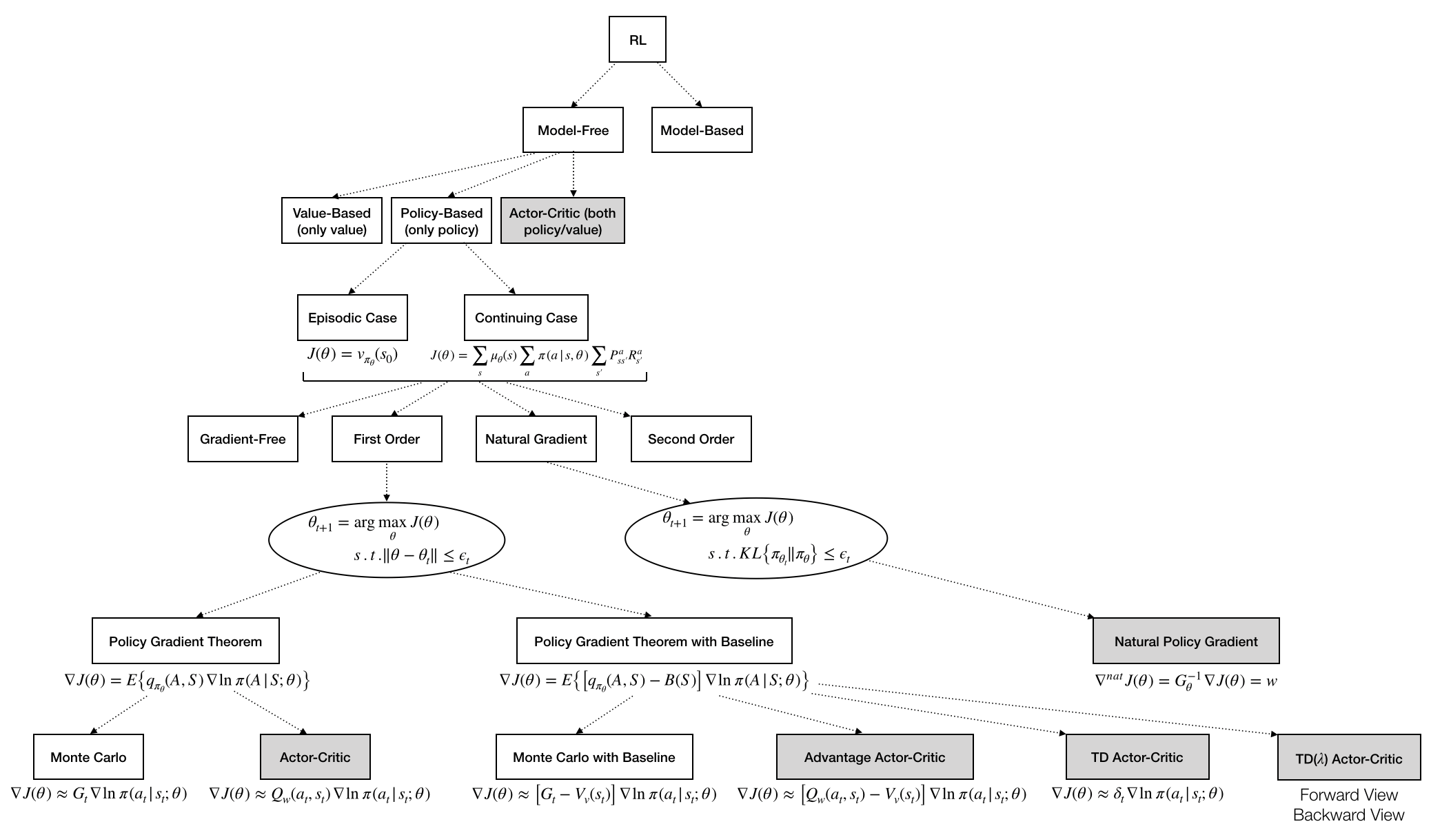
Policy-based algorithms use a parameterized policy, namely $\pi(a|s,\theta)$, while value-based algorithms use an $\epsilon$-greedy policy. This is a summary comparing the two classes of algorithms.

Algorithms	Advantages	Disadvantages
Value-based	Opposite to Policy-based	Opposite to Policy-based
Policy-based	1. Faster convergence (small change in $\theta$ translates into smooth change in policy) 2. No max operator (better for high-dimensional action space, continuous space) 3. Stochastic policy (in POMDPs or in contexts where the feature representation is not good enough stochastic policy may be optimal. Recall that for MDPs there is always an optimal policy)	1. Convergence to local optimum 2. High variance

Objectives for policy-based algorithms

There are two objectives (but there can be more, see Ideas at the end):

Objective for episodic case. Given an initial state $s_0$ we define

$$J(\theta)=v_{\pi_\theta}(\theta)$$

Objective for continuing case. Given an initial state $s_0$, we compute the average reward per time-step, namely

$$\begin{align} J(\theta) &= \lim_{h\rightarrow\infty}\frac{1}{h}\sum_{t=1}^h E\{r_t|\pi\} \\ &= \sum_s\mu_\theta(s)\sum_a\pi(a|s,\theta)\sum_{s'}P_{ss'}^aR_{s'}^a \quad\text{by ergodicity} \end{align}$$

Note that $J(\theta)$ is independent of the initial state. By definition of average reward, we redefine the state-value and the action-value functions in the following way:

$$\begin{align} v_{\pi_\theta}(s) &= E\{G_t|S_t=s\} \\ q_{\pi_\theta}(a,s) &= E\{G_t|S_t=s,A_t=a\} \\ G_t &= R_{t+1} - J(\theta) + \gamma\big(R_{t+2} - J(\theta)\big) + \dots \end{align}$$

Now that we have an objective, we can optimize it!
Question. How can we optimize it?
Answers. There are several classes of optimizers, namely:

1. Gradient-free methods, like finite difference policy gradient
2. First-order methods, which are based on an unbiased estimate of the gradient
   
   \[\begin{align} \theta_{t+1} = \arg & \max_\theta J(\theta) \\ & \text{s.t. } \|\theta-\theta_t\|\leq\epsilon_t \end{align}\]
   
3. Natural gradient methods, which are based on an unbiased estimate of the gradient under different assumptions from first-order methods
   
   \[\begin{align} \theta_{t+1} = \arg & \max_\theta J(\theta) \\ & \text{s.t. } KL\big\{\pi_{\theta_t}\|\pi_\theta\big\}\leq\epsilon_t \end{align}\]
   
4. Second-order methods, which takes into account the second order information

First-Order Methods

The Policy gradient theorem provides a way to estimate the gradient of $J(\theta)$. However, policy gradient algorithms have high variance. Later, we will consider a trick to deal with that, viz. using a baseline.

Policy Gradient Theorem

Theorem. Given an initial state $s_0$ and an objective function $J(\theta)$ (no matter if we are in the episodic or continuing case).

$$\nabla_\theta J(\theta) \propto E\big\{q_{\pi_\theta}(A,S)\nabla_\theta\ln\big(\pi(A|S,\theta)\big)\big\}$$

Proof. Firstly, we prove that $\nabla_\theta J(\theta) \propto \sum_s\mu_\theta(s)\sum_aq_{\pi_\theta}(a,s)\nabla_\theta\pi(a|s,\theta)$ for both the episodic and the continuing case.
Secondly we show that, $\sum_s\mu_\theta(s)\sum_aq_{\pi_\theta}(a,s)\nabla_\theta\pi(a|s,\theta)=E\big\{q_{\pi_\theta}(A,S)\nabla_\theta\ln\big(\pi(A|S,\theta)\big)\big\}$.
[Episodic case]. Let's consider the episodic case,

\[\begin{align} \nabla_\theta v_{\pi_\theta}(s) &= \nabla_\theta\sum_a\pi(a|s,\theta)q_{\pi_\theta}(a,s) \\ &= \sum_a\big\{\nabla_\theta\pi(a|s,\theta)q_{\pi_\theta}(a,s)+\pi(a|s,\theta)\nabla_\theta q_{\pi_\theta}(a,s)\big\} \\ &= \sum_a\big\{\nabla_\theta\pi(a|s,\theta)q_{\pi_\theta}(a,s)+\pi(a|s,\theta)\nabla_\theta \big[R_s^a+\sum_{s'}P_{ss'}^av_{\pi_\theta}(s')\big]\big\} \\ &= \sum_a\big\{\nabla_\theta\pi(a|s,\theta)q_{\pi_\theta}(a,s)+\pi(a|s,\theta)\sum_{s'}P_{ss'}^a\nabla_\theta v_{\pi_\theta}(s')\big\} \\ &= \sum_a\bigg\{\nabla_\theta\pi(a|s,\theta)q_{\pi_\theta}(a,s)+\pi(a|s,\theta) \\ &\quad\quad\sum_{s'}P_{ss'}^a\bigg[\sum_{a'}\big\{\nabla_\theta\pi(a'|s',\theta)q_{\pi_\theta}(a',s')+\pi(a'|s',\theta)\sum_{s^{''}}P_{s's^{''}}^{a'}\nabla_\theta v_{\pi_\theta}(s^{''})\big\}\bigg]\bigg\} \\ &= \sum_a\nabla_\theta\pi(a|s,\theta)q_{\pi_\theta}(a,s)+\sum_a\bigg\{\pi(a|s,\theta)\sum_{s'}P_{ss'}^a\sum_{a'}\nabla_\theta\pi(a'|s',\theta)q_{\pi_\theta}(a',s')\bigg\}+ \\ &\quad\quad\sum_a\bigg\{\pi(a|s,\theta)\sum_{s'}P_{ss'}^a\sum_{a'}\pi(a'|s',\theta)\sum_{s^{''}}P_{s's^{''}}^{a'}\nabla_\theta v_{\pi_\theta}(s^{''})\bigg\} \\ &= \sum_a\nabla_\theta\pi(a|s,\theta)q_{\pi_\theta}(a,s)+P(s\rightarrow s')\sum_{a'}\nabla_\theta\pi(a'|s',\theta)q_{\pi_\theta}(a',s')+ \\ &\quad\quad\sum_a\bigg\{\pi(a|s,\theta)\sum_{s'}P_{ss'}^a\sum_{a'}\pi(a'|s',\theta)\sum_{s^{''}}P_{s's^{''}}^{a'}\nabla_\theta v_{\pi_\theta}(s^{''})\bigg\} \\ &= \dots \quad \text{By expliciting the last term in recursive way} \\ &= \sum_{x\in S}\sum_{k=0}^\infty P(s\rightarrow x,k,\pi)\sum_a\nabla_\theta\pi(a|x,\theta)q_{\pi_\theta}(a,x) \\ &\quad\quad\text{where }P(s\rightarrow x,k,\pi)\text{ is the probability to go from s to x in k steps} \\ &= \sum_{x\in S}\eta(x)\sum_a\nabla_\theta\pi(a|x,\theta)q_{\pi_\theta}(a,x) \quad\text{where }\eta(x)=\sum_{k=0}^\infty P(s\rightarrow x,k,\pi) \\ &= \sum_{s\in S}\eta(s)\sum_a\nabla_\theta\pi(a|s,\theta)q_{\pi_\theta}(a,s) \\ &= \frac{\sum_{s'\in S}\eta(s')}{\sum_{s'\in S}\eta(s')}\sum_{s\in S}\eta(s)\sum_a\nabla_\theta\pi(a|s,\theta)q_{\pi_\theta}(a,s) \\ &= \sum_{s'\in S}\eta(s')\sum_{s\in S}\mu_\theta(s)\sum_a\nabla_\theta\pi(a|s,\theta)q_{\pi_\theta}(a,s) \quad\text{where }\mu_\theta(s)=\frac{\eta(s)}{\sum_{s'\in S}\eta(s')} \\ &\propto \sum_{s\in S}\mu_\theta(s)\sum_a\nabla_\theta\pi(a|s,\theta)q_{\pi_\theta}(a,s)\\ \end{align}\]

[Continuing case]. Let's consider the continuing case (note that in this case we cannot directly compute the gradient of $J(\theta)$ as the term $\mu_\theta(s)$ is unknwown),

$$\begin{align} \nabla_\theta v_{\pi_\theta}(s) &= \nabla_\theta\sum_a\pi(a|s,\theta)q_{\pi_\theta}(a,s) \\ &= \sum_a\big\{\nabla_\theta\pi(a|s,\theta)q_{\pi_\theta}(a,s)+\pi(a|s,\theta)\nabla_\theta q_{\pi_\theta}(a,s)\big\} \\ &= \sum_a\big\{\nabla_\theta\pi(a|s,\theta)q_{\pi_\theta}(a,s)+\pi(a|s,\theta)\nabla_\theta \big[R_s^a-J(\theta)+\sum_{s'}P_{ss'}^av_{\pi_\theta}(s')\big]\big\} \\ &= \sum_a\nabla_\theta\pi(a|s,\theta)q_{\pi_\theta}(a,s)-\nabla_\theta J(\theta)+\sum_a\pi(a|s,\theta)\sum_{s'}P_{ss'}^a\nabla_\theta v_{\pi_\theta}(s') \\ \end{align}$$

Now, we can explicit the gradient of $J(\theta)$, namely:

$$\nabla_\theta J(\theta)=\sum_a\nabla_\theta\pi(a|s,\theta)q_{\pi_\theta}(a,s)-\nabla_\theta v_{\pi_\theta}(s)+\sum_a\pi(a|s,\theta)\sum_{s'}P_{ss'}^a\nabla_\theta v_{\pi_\theta}(s')$$

In other words,

$$\begin{align} \nabla_\theta J(\theta) &= \sum_a\nabla_\theta\pi(a|s,\theta)q_{\pi_\theta}(a,s)-\nabla_\theta v_{\pi_\theta}(s)+\sum_a\pi(a|s,\theta)\sum_{s'}P_{ss'}^a\nabla_\theta v_{\pi_\theta}(s') \\ &= \sum_a\bigg[\nabla_\theta\pi(a|s,\theta)q_{\pi_\theta}(a,s)+\pi(a|s,\theta)\sum_{s'}P_{ss'}^a\nabla_\theta v_{\pi_\theta}(s')\bigg]-\nabla_\theta v_{\pi_\theta}(s) \\ \end{align}$$

Now we can sum both terms by $\sum_s\mu_\theta(s)$ (keep in mind that $\sum_s\mu_\theta(s)\nabla_\theta J(\theta)=\nabla_\theta J(\theta)$)

$$\begin{align} \nabla_\theta J(\theta) &= \sum_s\mu_\theta(s)\sum_a\bigg[\nabla_\theta\pi(a|s,\theta)q_{\pi_\theta}(a,s)+\pi(a|s,\theta)\sum_{s'}P_{ss'}^a\nabla_\theta v_{\pi_\theta}(s')\bigg]-\sum_s\mu_\theta(s)\nabla_\theta v_{\pi_\theta}(s) \\ &= \sum_s\mu_\theta(s)\sum_a\nabla_\theta\pi(a|s,\theta)q_{\pi_\theta}(a,s)+\sum_s\mu_\theta(s)\sum_a\pi(a|s,\theta)\sum_{s'}P_{ss'}^a\nabla_\theta v_{\pi_\theta}(s')-\sum_s\mu_\theta(s)\nabla_\theta v_{\pi_\theta}(s) \\ &= \sum_s\mu_\theta(s)\sum_a\nabla_\theta\pi(a|s,\theta)q_{\pi_\theta}(a,s)+\sum_{s'}\sum_s\mu_\theta(s)\sum_a\pi(a|s,\theta)P_{ss'}^a\nabla_\theta v_{\pi_\theta}(s')-\sum_s\mu_\theta(s)\nabla_\theta v_{\pi_\theta}(s) \\ &= \sum_s\mu_\theta(s)\sum_a\nabla_\theta\pi(a|s,\theta)q_{\pi_\theta}(a,s)+\sum_{s'}\sum_s\mu_\theta(s)P(s\rightarrow s')\nabla_\theta v_{\pi_\theta}(s')-\sum_s\mu_\theta(s)\nabla_\theta v_{\pi_\theta}(s) \\ &\quad\quad\text{where }P(s\rightarrow s')=\sum_a\pi(a|s,\theta)P_{ss'}^a \\ &= \sum_s\mu_\theta(s)\sum_a\nabla_\theta\pi(a|s,\theta)q_{\pi_\theta}(a,s)+\sum_{s'}\mu_\theta(s')\nabla_\theta v_{\pi_\theta}(s')-\sum_s\mu_\theta(s)\nabla_\theta v_{\pi_\theta}(s) \\ &\quad\quad\text{recall that }\sum_s\mu_\theta(s)P(s\rightarrow s')=\mu_\theta(s') \\ &= \sum_s\mu_\theta(s)\sum_a\nabla_\theta\pi(a|s,\theta)q_{\pi_\theta}(a,s) \end{align}$$

[Last step].

$$\begin{align} \nabla_\theta J(\theta) &\propto \sum_s\mu_\theta(s)\sum_aq_{\pi_\theta}(a,s)\nabla_\theta\pi(a|s,\theta) \\ &= E\big\{\sum_aq_{\pi_\theta}(a,S)\nabla_\theta\pi(a|S,\theta)\big\} \\ &\quad\quad\text{we have defined random variable S and compute its expectation conditioned on initial state }s_0 \\ &= E\bigg\{\sum_a\pi(a|S,\theta)q_{\pi_\theta}(a,S)\frac{\nabla_\theta\pi(a|S,\theta)}{\pi(a|S,\theta)}\bigg\} \\ &= E\bigg\{q_{\pi\theta}(A,S)\frac{\nabla_\theta\pi(A|S,\theta)}{\pi(A|S,\theta)}\bigg\} \quad\text{similarly, we have defined random variable A}\\ &= E\big\{q_{\pi_\theta}(A,S)\nabla_\theta\ln\pi(A|S,\theta)\big\}\\ \end{align}$$ QED

Estimate 1: Monte Carlo Policy Gradient (REINFORCE)

$$\begin{align} \nabla_\theta J(\theta) &\propto E\big\{q_{\pi\theta}(A,S)\nabla_\theta\ln\pi(A|S,\theta)\big\}\\ &= E\big\{E\{G_t|A'=A,S'=S\}\nabla_\theta\ln\pi(A|S,\theta)\big\}\\ &= E\big\{G\nabla_\theta\ln\pi(A|S,\theta)\big\} \quad\text{as }E\{G|A'=A,S'=S\}=P(A'=A,S'=S)G=G \\ &\approx g_t\nabla_\theta\ln\pi(a|s,\theta) \end{align}$$

Note that this algorithm works only in the episodic case, since we need the return, which is available only at the end. The return is a summation of all rewards and therefore it introduces a lot of variance.

Estimate 2: Actor-Critic Policy Gradient

Another strategy (which has less variance) can be obtained by using an action-value function approximator

$$\begin{align} \nabla_\theta J(\theta) &\propto E\big\{q_{\pi\theta}(A,S)\nabla_\theta\ln\pi(A|S,\theta)\big\}\\ &\approx Q_w(a,s)\nabla_\theta\ln\pi(a|s,\theta) \end{align}$$

Therefore, we can leverage all knowledge we have to perform policy evaluation to learn $Q_w(a,s)$ and then learn the policy function approximator.

Policy Gradient Theorem with Baseline

Theorem. Given an initial state $s_0$ and an objective function $J(\theta)$ (no matter if we are in the episodic or continuing case). $$\nabla_\theta J(\theta) \propto E\big\{\big(q_{\pi_\theta}(A,S)-v_{\pi_\theta}(S)\big)\nabla_\theta\ln\big(\pi(A|S,\theta)\big)\big\}$$

Proof. We can extend the normal policy gradient theorem, by introducing a baseline function $B(s)$, namely

$$\begin{align} E\big\{B(S)\nabla_\theta\ln\pi_\theta(A|S)\big\} &= \sum_s\mu_\theta(s)\sum_a\pi(a|s,\theta)B(S)\nabla_\theta\ln\pi_\theta(A|S) \\ &= \sum_s\mu_\theta(s)B(S)\sum_a\pi(a|s,\theta)\nabla_\theta\ln\pi_\theta(A|S) \\ &= \sum_s\mu_\theta(s)B(S)\sum_a\nabla_\theta\pi_\theta(A|S) \\ &= \sum_s\mu_\theta(s)B(S)\nabla_\theta\sum_a\pi_\theta(A|S) \\ &= \sum_s\mu_\theta(s)B(S)\nabla_\theta 1 \\ &= 0 \end{align}$$

This result is valid for any baseline function. Let's choose $B(s)=v_{\pi_\theta}(s)$. The result of the theorem follows in straightforward way. QED

Note that $q_{\pi_\theta}(a,s)-v_{\pi_\theta}(s)$ is usually called the advantage function (as it measures what is the contribution of action a with respect to the expected value).

Estimate 1: Monte Carlo Policy Gradient with Baseline

$$\begin{align} \nabla_\theta J(\theta) &\propto E\big\{\big(q_{\pi_\theta}(A,S)-v_{\pi_\theta}(S)\big)\nabla_\theta\ln\big(\pi(A|S,\theta)\big)\big\} \\ &\approx \big(g-V_v(s)\big)\nabla_\theta\ln\big(\pi(a|s,\theta)\big) \end{align}$$

Variance can be still reduced. Furthemore, we need to wait until the end of episode.

Estimate 2: Advantage Actor-Critic Policy Gradient

$$\begin{align} \nabla_\theta J(\theta) &\propto E\big\{\big(q_{\pi_\theta}(A,S)-v_{\pi_\theta}(S)\big)\nabla_\theta\ln\big(\pi(A|S,\theta)\big)\big\} \\ &\approx \big(Q_w(a,s)-V_v(s)\big)\nabla_\theta\ln\big(\pi(a|s,\theta)\big) \end{align}$$

The problem of this approach is that we need three function approximators (lots of parameters). See next estimate for using only two. Alternatively, check ideas.

Estimate 3: TD Actor-Critic Policy Gradient

$$\begin{align} \nabla_\theta J(\theta) &\propto E\big\{\big(q_{\pi_\theta}(A,S)-v_{\pi_\theta}(S)\big)\nabla_\theta\ln\big(\pi(A|S,\theta)\big)\big\} \\ &= E\big\{\big(E\{G|\tilde{A}=A,\tilde{S}=S\}-v_{\pi_\theta}(S)\big)\nabla_\theta\ln\big(\pi(A|S,\theta)\big)\big\} \\ &= E\big\{\big(E\{R+\gamma v_{\pi_\theta}(S')|\tilde{A}=A,\tilde{S}=S\}-v_{\pi_\theta}(S)\big)\nabla_\theta\ln\big(\pi(A|S,\theta)\big)\big\} \\ &= E\big\{\big(E\{R+\gamma v_{\pi_\theta}(S')-v_{\pi_\theta}(\tilde{S})|\tilde{A}=A,\tilde{S}=S\}\big)\nabla_\theta\ln\big(\pi(A|S,\theta)\big)\big\} \\ &= E\big\{\big(R+\gamma v_{\pi_\theta}(S')-v_{\pi_\theta}(S)\big)\nabla_\theta\ln\big(\pi(A|S,\theta)\big)\big\} \\ &\approx \big(R+\gamma V_v(s')-V_v(s)\big)\nabla_\theta\ln\big(\pi(a|s,\theta)\big) \\ \end{align}$$

Estimate 4: TD($\lambda$) Actor-Critic Policy Gradient (Forward View)

$$\begin{align} \nabla_\theta J(\theta) &\propto E\big\{\big(q_{\pi_\theta}(A,S)-v_{\pi_\theta}(S)\big)\nabla_\theta\ln\big(\pi(A|S,\theta)\big)\big\} \\ &\approx \big(g^\lambda-V_v(s)\big)\nabla_\theta\ln\big(\pi(a|s,\theta)\big) \\ \end{align}$$

In this case, we need to wait until the end of the episode.

Estimate 5: TD($\lambda$) Actor-Critic Policy Gradient (Forward View)

$$\begin{align} \nabla_\theta J(\theta) &\propto E\big\{\big(q_{\pi_\theta}(A,S)-v_{\pi_\theta}(S)\big)\nabla_\theta\ln\big(\pi(A|S,\theta)\big)\big\} \\ &\approx \big(R+\gamma V_v(s')-V_v(s)\big)e \\ \end{align}$$

where

$$e\leftarrow \lambda e+\nabla_\theta\ln\pi(a|s,\theta)$$

is the eligibility trace.

Summary of First-Order Gradient Methods

Name	Formula	Baseline	Episodic	Continuing	Parameters	Variance	Bias
Monte-Carlo (REINFORCE)	\(\nabla_\theta J(\theta)\approx g_t\nabla_\theta\ln\pi(a|s,\theta)\)	No	Yes	No	1	High	Low
Actor-Critic	\(\nabla_\theta J(\theta)\approx Q_w(a,s)\nabla_\theta\ln\pi(a|s,\theta)\)	No	Yes	Yes	2	Medium	Medium (but can be Low)
Monte Carlo with Baseline	\(\nabla_\theta J(\theta)\approx \big(g-V_v(s)\big)\nabla_\theta\ln\pi(a|s,\theta)\)	Yes	Yes	No	2	Medium	Low
Advantage Actor-Critic	\(\nabla_\theta J(\theta)\approx \big(Q_w(a,s)-V_v(s)\big)\nabla_\theta\ln\pi(a|s,\theta)\)	Yes	Yes	Yes	3	Low	Medium (but can be Low)
TD Actor-Critic	\(\nabla_\theta J(\theta)\approx \big(R+\gamma V_v(s')-V_v(s)\big)\nabla_\theta\ln\pi(a|s,\theta)\)	Yes	Yes	Yes	2	Low	Medium
TD(\(\lambda\)) Actor-Critic (Forward)	\(\nabla_\theta J(\theta)\approx \big(g^\lambda-V_v(s)\big)\nabla_\theta\ln\pi(a|s,\theta)\)	Yes	Yes	No	2	Low-Medium (tradeoff)	Low-Medium (tradeoff)
TD(\(\lambda\)) Actor-Critic (Backward)	\(\nabla_\theta J(\theta)\approx \big(R+\gamma V_v(s')-V_v(s)\big)e\) \(e\leftarrow \lambda e+\nabla_\theta\ln\pi(a|s,\theta)\)	Yes	Yes	Yes	2	Low-Medium (tradeoff)	Low-Medium (tradeoff)

Natural Gradient Methods

Firstly, we show some properties of the KL divergence. Secondly, we derive the update rule of natural gradient algorithms. Thirdly, we derive the natural policy gradient algorithm.

Properties of KL Divergence

We try to use similar notation used so far. For example, we use $\pi(a|\theta)$ to refer to $\pi(a|s,\theta)$ in the context of policy gradient algorithms. More generally, we can think of $\pi(a|\theta)$ to any arbitrary density parameterized by vector $\theta$. We show that KL divergence can be approximated in the following way:

$$\begin{align} KL\big\{\pi_{\theta_t}\|\pi_\theta\} &\approx \Delta\theta^TG(\theta_t)\Delta\theta \\ G(\theta) &= E_A\big\{\nabla_\theta\ln\pi(A|\theta)\nabla_\theta\ln\pi(A|\theta)^T\big\} \\ \Delta\theta &= \theta-\theta_t \end{align}$$

for $\|\Delta\theta\|\rightarrow 0$.
Let's derive this approximation ($\pi_\theta(\cdot)\doteq\pi(\cdot|\theta)$)

$$\begin{align} KL\big\{\pi_{\theta_t}\|\pi_\theta\} &= \int \pi_{\theta_t}(a)\ln\frac{\pi_{\theta_t}(a)}{\pi_\theta(a)}da \\ &=-\int \pi_{\theta_t}(a)\ln\frac{\pi_\theta(a)}{\pi_{\theta_t}(a)}da \\ &=-\int \pi_{\theta_t}(a)\ln\frac{\Delta p(a)+\pi_{\theta_t}(a)}{\pi_{\theta_t}(a)}da \quad\text{where }\Delta p=\pi_\theta-\pi_{\theta_t} \\ &=-\int \pi_{\theta_t}(a)\ln\bigg\{1+\frac{\Delta p(a)}{\pi_{\theta_t}(a)}\bigg\}da \\ &\approx-\int \pi_{\theta_t}(a)\bigg\{\frac{\Delta p(a)}{\pi_{\theta_t}(a)}-\frac{1}{2}\bigg[\frac{\Delta p(a)}{\pi_{\theta_t}(a)}\bigg]^2\bigg\}da \quad\text{where we use Taylor expansion }\ln(1+x)=x-\frac{x^2}{2}+O(x^2)\\ &=-\int \pi_{\theta_t}(a)\frac{\Delta p(a)}{\pi_{\theta_t}(a)}da+\frac{1}{2}\int \pi_{\theta_t}(a)\bigg[\frac{\Delta p(a)}{\pi_{\theta_t}(a)}\bigg]^2da \\ &=-\int \Delta p(a)da+\frac{1}{2}\int \pi_{\theta_t}(a)\bigg[\frac{\Delta p(a)}{\pi_{\theta_t}(a)}\bigg]^2da \\ &\approx-\int \nabla_\theta\pi_{\theta_t}(a)^T\Delta\theta da+\frac{1}{2}\int \pi_{\theta_t}(a)\bigg[\frac{\Delta p(a)}{\pi_{\theta_t}(a)}\bigg]^2da \quad\text{note that }\Delta p(a)\approx\nabla_\theta\pi_{\theta_t}(a)^T\Delta\theta\\ &=-\bigg[\int \nabla_\theta\pi_{\theta_t}(a)^T da\bigg]\Delta\theta+\frac{1}{2}\int \pi_{\theta_t}(a)\bigg[\frac{\Delta p(a)}{\pi_{\theta_t}(a)}\bigg]^2da \\ &=-\bigg[\int \nabla_\theta\pi_{\theta_t}(a) da\bigg]^T\Delta\theta+\frac{1}{2}\int \pi_{\theta_t}(a)\bigg[\frac{\Delta p(a)}{\pi_{\theta_t}(a)}\bigg]^2da \\ &=-\bigg[\nabla_\theta\int \pi_{\theta_t}(a) da\bigg]^T\Delta\theta+\frac{1}{2}\int \pi_{\theta_t}(a)\bigg[\frac{\Delta p(a)}{\pi_{\theta_t}(a)}\bigg]^2da \\ &=-\bigg[\nabla_\theta 1\bigg]^T\Delta\theta+\frac{1}{2}\int \pi_{\theta_t}(a)\bigg[\frac{\Delta p(a)}{\pi_{\theta_t}(a)}\bigg]^2da \\ &=\frac{1}{2}\int \pi_{\theta_t}(a)\bigg[\frac{\Delta p(a)}{\pi_{\theta_t}(a)}\bigg]^2da \\ &=\frac{1}{2}E_A\bigg\{\bigg[\frac{\Delta p(a)}{\pi_{\theta_t}(a)}\bigg]^2\bigg\} \\ &=\frac{1}{2}E_A\big\{\Delta\theta^T\nabla_\theta\ln\pi(A|\theta_t)\nabla_\theta\ln\pi(A|\theta_t)^T\Delta\theta\big\} \quad\text{where we use Taylor expansion as before }\frac{\Delta p(A)}{\pi_{\theta_t}(A)}\approx \frac{\nabla_\theta\pi_{\theta_t}(A)^T\Delta\theta}{\pi_{\theta_t}(A)}=\frac{\sum_i\frac{\partial\pi_{\theta_t}(A)}{\partial\theta_i}\Delta\theta_i}{\pi_{\theta_t}(A)}=\sum_i\frac{\partial\ln\pi_{\theta_t}(A)}{\partial\theta_i}\Delta\theta_i = \nabla_\theta\ln\pi_{\theta_t}(A)^T\Delta\theta = \nabla_\theta\ln\pi(A|\theta_t)^T\Delta\theta \\ &=\frac{1}{2}\Delta\theta^TE_A\big\{\nabla_\theta\ln\pi(A|\theta_t)\nabla_\theta\ln\pi(A|\theta_t)^T\big\}\Delta\theta \\ &=\frac{1}{2}\Delta\theta^TG(\theta_t)\Delta\theta \end{align}$$

Update Rule for Natural Gradient Algorithms

The update rule is derived from the following constrained optimization problem

$$\begin{align} \theta_{t+1} = \arg & \min_\theta -J(\theta) \\ & \text{s. t. } \frac{1}{2}\Delta\theta^TG(\theta_t)\Delta\theta\leq\epsilon_t \end{align}$$

Let's consider the Lagrangian

$$\begin{align} \mathcal{L}(\theta,\lambda_t) &= -J(\theta) + \lambda_t\bigg[\frac{1}{2}\Delta\theta^TG(\theta_t)\Delta\theta-\epsilon_t\bigg] \\ &\approx -J(\theta_t) - \nabla_\theta J(\theta_t)^T\Delta\theta + \lambda_t\bigg[\frac{1}{2}\Delta\theta^TG(\theta_t)\Delta\theta-\epsilon_t\bigg] \\ &\quad\quad\text{where we use the Taylor approximation for }J(\theta) \\ &= - J(\theta_t) - \nabla_\theta J(\theta_t)^T(\theta-\theta_t) + \lambda_t\bigg[\frac{1}{2}(\theta-\theta_t)^TG(\theta_t)(\theta-\theta_t)-\epsilon_t\bigg] \\ \end{align}$$

Now, let's compute the gradient with respect to $\theta$ and equate it to 0.

$$\begin{align} \nabla_\theta\mathcal{L}(\theta,\lambda_t) &\approx -\nabla_\theta J(\theta_t) + \lambda_tG(\theta_t)(\theta-\theta_t)=0 \end{align}$$

which give us the update rule

$$\theta=\theta_t+\frac{G(\theta_t)^{-1}}{\lambda_t}\nabla_\theta J(\theta_t)$$

Therefore,

$$\nabla_\theta^{nat}J(\theta_t)=G(\theta_t)^{-1}\nabla_\theta J(\theta_t)$$

Natural Policy Gradient Algorithm

Given an action value approximator $Q_w(a,s)=\nabla_\theta\ln\pi(a|s,\theta)^Tw$ (which is called compatible function approximator, as $\nabla_wQ_w(a,s)=\nabla_\theta\ln\pi(a|s,\theta)$), we have that

$$\nabla_\theta^{nat}J(\theta_t)\propto w_t$$

In fact, assume that $Q_w(a,s)=q_{\pi_\theta}(a,s)$

$$\begin{align} \nabla_\theta J(\theta) &\propto E\big\{q_{\pi\theta}(A,S)\nabla_\theta\ln\pi(A|S,\theta)\big\} \\ &= E\big\{\nabla_\theta\ln\pi(A|S,\theta)Q_w(A,S)\big\} \\ &= E\big\{\nabla_\theta\ln\pi(A|S,\theta)\nabla_\theta\ln\pi(a|s,\theta)^Tw\big\} \\ &= E\big\{\nabla_\theta\ln\pi(A|S,\theta)\nabla_\theta\ln\pi(a|s,\theta)^T\big\}w \\ &= G(\theta)w \\ \end{align}$$

Now by the result of previous section

$$\begin{align} \nabla_\theta^{nat}J(\theta_t) &= G(\theta_t)^{-1}\nabla_\theta J(\theta_t) \\ &\propto G(\theta_t)^{-1}G(\theta_t)w_t \\ &\propto w_t \end{align}$$

Therefore, using a compatible function approximator allows to avoid to compute $G(\theta_t)$ and its inverse.